Download
1 / 44
440 likes | 551 Views
Bioinformatics 3 V 3 – Data for Building Networks. Fri, Oct 25, 2013. Graph Layout 1. Requirements : • fast and stable • nice graphs • visualize relations • symmetry • interactive exploration • …. Force-directed Layout: based on energy minimization → runtime → mapping into 2D.

E N D
Bioinformatics 3V 3 – Data for Building Networks Fri, Oct 25, 2013
Graph Layout 1 Requirements: • fast and stable • nice graphs • visualize relations • symmetry • interactive exploration • … Force-directed Layout: based on energy minimization → runtime → mapping into 2D H3: for hierarchic graphs → MST-based cone layout → hyperbolic space → efficient layout for biological data???
Aim: analyze and visualize homologies within the protein universe 50 genomes, 145579 proteins, 21 × 109 BLASTP pairwise sequence comparisons Expectations: • homologs will be close together • fusion proteins („Rosetta Stone proteins“) will link proteins of related function. → need to visualize an extremely large network! → develop a stepwisescheme
LGL: stepwise scheme (0) create network from BLAST E-score 145'579 proteins E < 10–12 → 1'912'684 links , 30737 proteins in the largest cluster (1) separate original network into connected sets 11517 connected components, 33975 proteins w/out links (2) force directed layout of each component independently, based on a MST (3) integrate connected sets into one coordinate system via a funnel process, starting from the largest set The first connected set is placed at the bottom of a potential funnel. Other sets are placed one at a time on the rim of the potential funnel and allowed to fall towards the bottom where they are frozen in space upon collision with the previous sets. Adai et al. J. Mol. Biol. 340, 179 (2004)
Component layout I For each component independently: → start from the root node of the MST assigned arbitrarily (educated guess) most "central" node Centrality: minimize total distance to all other nodes in the component Level n-nodes: nodes that are n links away from the root in the MST Layout → place root at the center
Component Layout II • start with root node of the MST • place level-1 nodes on circle (sphere) around root, add all links, relax springs (+ short-range repulsion) • place level-2 nodes on circles (sphere) outside their level-1 descendants, add all links, relax springs • place level-3 nodes on circles (sphere) outside their level-2 descendants, : Adai et al. J. Mol. Biol. 340, 179 (2004)
Combining the Components When the components are finished assemble using energy funnel • place largest component at bottom • place next smaller one somewhere on the rim, let it slide down freeze upon contact No information in the relative positions of the components!!! Adai et al. J. Mol. Biol. 340, 179 (2004)
Annotations in the Largest Cluster Related functions in the same regions of the cluster → predictions Adai et al. J. Mol. Biol. 340, 179 (2004)
Clustering of Functional Classes Adai et al. J. Mol. Biol. 340, 179 (2004)
Fusion Proteins Fusion proteins connect two protein homology families A, A', A'', AB and B, B', AB historic genetic events: fusion, fission, duplications, … Also in the network: homologies <=> edges remote homologies <=> in the same cluster non-homologous functional relations <=> adjacent, linked clusters Adai et al. J. Mol. Biol. 340, 179 (2004)
Functional Relations between Gene Families Examples of spatial localization of protein function in the map A: the linkage of the tryptophan synthase α family to the functionally coupled but non-homologous β family by the yeast tryptophan synthase αβ fusion protein, B: protein subunits of the pyruvate synthase and alpha-ketoglutarate ferredexin oxidoreductase complexes C: metabolic enzymes, particularly those of acetyl CoA and amino acid metabolism DUF213 likely has metabolic function! Adai et al. J. Mol. Biol. 340, 179 (2004)
And the Winner iiiis… Compare the layouts from A: LGL – hierarchic force-directed layout according to MST structure from homology B: globalforce-directed layout without MST no structure, no components visible C: InterViewer – collapses similar nodes reduced complexity Adai et al. J. Mol. Biol. 340, 179 (2004)
Graph Layout: Summary Approach Idea Force-directed spring model relax energy, springs of appropriate lengths the same physical concept, different implementations! relax energy, springs for links, Coulomb repulsion between all nodes Force-directed spring-electric model H3 spanning tree in hyperbolic space hierarchic, force-directed algorithm for modules LGL
what are interesting biological "things"? how are they connected? are the informations accessible/reliable? Vertices = the "things" to be connected "Graph" = more than the sum of the individual parts ???? Edges = encode the connectivity Classified by: • degree distribution • clustering • connected components • … A "Network" So far: G = (E, V)
Protein Complexes Complex formation may lead to modification of the active site Assembly of structures protein machinery built from parts via dimerization and oligomerization Complex formation may lead to increased diversity Cooperation and allostery
Gel Electrophoresis Electrophoresis: directed diffusion of charged particles in an electric field faster Higher charge, smaller Lower charge, larger slower Put proteins in a spot on a gel-like matrix, apply electric field separation according to size (mass) and charge identify constituents of a complex Nasty details: protein charge vs. pH, cloud of counter ions, protein shape, denaturation, …
SDS-PAGE For better control: denature proteins with detergent Often used: sodium dodecyl sulfate (SDS) denatures and coats the proteins with a negative charge charge proportional to mass traveled distance per time SDS-polyacrylamide gel electrophoresis After the run: staining to make proteins visible For "quantitative" analysis: compare to marker (set of proteins with known masses) Image from Wikipedia, marker on the left lane
P pH Protein Charge? Main source for charge differences: pH-dependent protonation states <=> Equilibrium between • density (pH) dependent H+-binding and • density independent H+-dissociation Probability to have a proton: pKa = pH value for 50% protonation Asp 3.7–4.0 … His 6.7–7.1 … Lys 9.3-9.5 Each H+ has a +1e charge Isoelectric point: pH at which the protein is uncharged protonation state cancels permanent charges
2D Gel Electrophoresis Two steps: i) separation by isoelectric point via pH-gradient ii) separation by mass with SDS-PAGE low pH high pH Step 1: protonated => pos. charge unprotonated => neg. charge Step 2: SDS-Page Most proteins differ in mass and isoelectric point (pI)
Mass Spectrometry Identify constituents of a (fragmented) complex via their mass patterns, detect by pattern recognition with machine learning techniques. http://gene-exp.ipk-gatersleben.de/body_methods.html
Tandem affinity purification Yeast 2-Hybrid-method can only identify binary complexes. In affinity purification, a protein of interest (bait) is tagged with a molecular label (dark route in the middle of the figure) to allow easy purification. The tagged protein is then co-purified together with its interacting partners (W–Z). This strategy can also be applied on a genome scale. Identify proteins by mass spectro- metry (MALDI- TOF). Gavin et al. Nature 415, 141 (2002)
TAP analysis of yeast PP complexes Identify proteins by scanning yeast protein database for protein composed of fragments of suitable mass. Here, the identified proteins are listed according to their localization (a). (b) lists the number of proteins per complex. Gavin et al. Nature 415, 141 (2002)
Validation of TAP methodology Check of the method: can the same complex be obtained for different choices of attachment point (tag protein attached to different coponents of complex)? Yes, more or less (see gel in (a)). Gavin et al. Nature 415, 141 (2002)
Pros and Cons Advantages: • quantitative determination of complex partners in vivo without prior knowledge • simple, high yield, high throughput Difficulties: • tag may prevent binding of the interaction partners • tag may change (relative) expression levels • tag may be buried between interaction partners → no binding to beads
Yeast Two-Hybrid Screening Discover binary protein-protein interactions via physical interaction complex of binding domain (BD) + activator domain (AD) fuse bait to BD, prey to AD → expression only when bait:prey-complex
Performance of Y2H Advantages: • in vivo test for interactions • cheap + robust → large scale tests Problems: • investigate the interaction between (i) overexpressed (ii) fusion proteins in the (iii) yeast (iv) nucleus many false positives (up to 50% errors) • spurious interactions via third protein
Synthetic Lethality Apply two mutations that are viable on their own, but lethal when combined. In cancer therapy, this effect implies that inhibiting one of these genes in a context where the other is defective should be selectively lethal to the tumor cells but not toxic to the normal cells, potentially leading to a large therapeutic window. http://jco.ascopubs.org/ Synthetic lethality may point to: • physical interaction (building blocks of a complex) • both proteins belong to the same pathway • both proteins have the same function (redundancy)
Gene Coexpression All constituents of a complex should be present at the same point in the cell cycle test for correlated expression No direct indication for complexes (too many co-regulated genes), but useful "filter"-criterion Standard tool: DNA micro arrays DeRisi, Iyer, Brown, Science278 (1997) 680: Diauxic shift from fermentation to respiration in S. cerevisiae Identify groups of genes with similar expression profiles
DNA Microarrays Fluorescence labeled DNA (cDNA) applied to micro arrays hybridization with complementary library strand fluorescence indicates relative cDNA amounts two labels (red + green) for experiment and control Usually: red = signal green = control yellow = "no change"
Diauxic Shift image analysis + clustering Identify groups of genes with similar time courses = expression profiles "cause or correlation"? — biological significance? DeRisi, Iyer, Brown, Science278 (1997) 680
Interaction Databases Bioinformatics: make use of existing databases
TAP Y2H annotated: septin complex HMS-PCI (low) Overlap of Results For yeast: ~ 6000 proteins => ~18 million potential interactions rough estimates: ≤ 100000 interactions occur 1 true positive for 200 potential candidates = 0.5% decisive experiment must have accuracy << 0.5% false positives Different experiments detect different interactions For yeast: 80000 interactions known, 2400 found in > 1 experiment Problems with experiments: i) incomplete coverage ii) (many) false positives iii) selective to type of interaction and/or compartment see: von Mering (2002)
Criteria for Reliability Guiding principles (incomplete list!): 1) mRNA abundance: most experimental techniques are biased towards high-abundance proteins 2) compartments: • most methods have their "preferred compartment" • proteins from same compartment => more reliable 3) co-functionality complexes have a functional reason (assumption!?)
In-Silico Prediction Methods Sequence-based: • gene clustering • gene neighborhood • Rosetta stone • phylogenetic profiling • coevolution Structure-based: • interface propensities • spatial simulations "Work on the parts list" fast unspecific high-throughput methods for pre-sorting "Work on the parts" specific, detailed expensive accurate
Gene Clustering Idea: functionally related proteins or parts of a complex are expressed simultaneously Search for genes with a common promoter when activated, all are transcribed together as one operand Example: bioluminescence in V. fischeri, regulated via quorum sensing three proteins: I, AB, CDE
genome 1 genome 2 genome 3 Gene Neighborhood Hypothesis again: functionally related genes are expressed together "functionally" = same {complex | pathway | function | …} Search for similarsequences of genes in differentorganisms (<=> Gene clustering: one species, promoters)
sp 1 sp 2 sp 3 sp 4 sp 5 Rosetta Stone Method Idea: same "names" in different genome "texts" Enright, Ouzounis (2001): 40000 predicted pair-wise interactions from search across 23 species Multi-lingual stele from 196 BC, found by the French in 1799 key to deciphering hieroglyphs
Phylogenetic Profiling Idea: either all or none of the proteins of a complex should be present in an organism compare presence of protein homologs across species (e.g., via sequence alignment)
Distances Hamming distance between species: number of different protein occurrences Two pairs with similar occurrence: P2-P7 and P3-P6
Coevolution Idea: not only similar static occurence, but similar dynamicevolution Interfaces of complexes are often better conserved than the rest of the protein surfaces. Also: look for potential substitutes anti-correlated missing components of pathways function prediction across species novel interactions
i2h method Schematic representation of the i2h method. A: Family alignments are collected for two different proteins, 1 and 2, including corresponding sequences from different species (a, b, c, ). B: A virtual alignment is constructed, concatenating the sequences of the probable orthologous sequences of the two proteins. Correlated mutations are calculated. Pazos, Valencia, Proteins 47, 219 (2002)
Correlated mutations at interface Correlated mutations evaluate the similarity in variation patterns between positions in a multiple sequence alignment. Similarity of those variation patterns is thought to be related to compensatory mutations. Calculate for each positions i and jin the sequence a rank correlation coefficient (rij): where the summations run over every possible pair of proteins k and l in the multiple sequence alignment. Siklis the ranked similarity between residue i in protein k and residue i in protein l. Sjkl is the same for residue j. Si and Sj are the means of Sikland Sjkl. Pazos, Valencia, Proteins 47, 219 (2002)
Summary What you learned today: how to get some data on PP interactions gene clustering SDS-PAGE TAP DB gene neighborhood MS micro array Y2H Rosetta stone synthetic lethality phylogenic profiling coevolution type of interaction? — reliability? — sensitivity? — coverage? — … Nextlecture: Mon, Oct. 28, 2013 • combining weak indicators: Bayesian analysis • identifying communities in networks