NETWORK MODELS
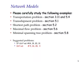
NETWORK MODELS. Networks. Physical Networks Road Networks Railway Networks Airline traffic Networks Electrical networks, e.g., the power grid Abstract networks organizational charts precedence relationships in projects Others?. Network Overview.


NETWORK MODELS
E N D
Presentation Transcript
Networks • Physical Networks • Road Networks • Railway Networks • Airline traffic Networks • Electrical networks, e.g., the power grid • Abstract networks • organizational charts • precedence relationships in projects • Others? NETWORK MODELS
Network Overview • Networks and graphs are powerful modeling tools. • Most OR models have networks or graphs as a major aspect • Each representation has its advantages • Major purpose of a representation • efficiency in algorithms • ease of use NETWORK MODELS
Algorithms Discussed • Minimal Spanning Tree • Shortest route algorithm • Maximum Flow Algorithm • Minimum Cost Capacitated Network • Critical Path Method NETWORK MODELS
Basic Definitions • A graph or network is defined by two sets of symbols: • Nodes: A set of points or vertices(call it V) are called nodes of a graph or network. • Arcs: An arc consists of an ordered pair of vertices and represents a possible direction of motion that may occur between vertices. Nodes 1 2 Arc 1 2 NETWORK MODELS
Basic Definitions • A network consists of nodes and arcs and the notation followed is • N = {1,2,3,4} • A = {(1,2), (1,3), (2,3), (2,4), (3,4)} 3 1 4 2 NETWORK MODELS
Basic Definitions • The flow in a network is limited by the capacity of arc (may be infinite also) • An arc is said to be directed if the flow is allowed in only one direction. • A path is a sequence of distinct branches that join two nodes regardless of direction of flow. • A path forms a loop or cycle if it connects a node to itself. • A directed loop or a circuit is a loop in which all the branches are oriented in the same direction. • A connected network is such that every two distinct nodes are linked by at least one path. • A spanning tree links all the nodes of the network with no loops allowed. NETWORK MODELS
Basic Definitions • Path / Connected nodes • Path :a collection of arcs formed by a series of adjacent nodes. • The nodes are said to be connected if there is a path between them. • Cycles / Trees / Spanning Trees • Cycle : a path starting at a certain node and returning to the same node without using any arc twice. • Tree : a series of nodes that contain no cycles. • Spanning tree : a tree that connects all the nodes in a network ( it consists of n -1 arcs). NETWORK MODELS
Network model & LP Model • Every network model has an underlying linear programming model • For every node there is exactly one constraint • For every arc there is one decision variable Xij, where i is the starting node and j is the ending node NETWORK MODELS
Minimal Spanning Tree • This algorithm deals with linking the nodes of network, directly or indirectly, using the shortest length of connecting branches. • Application are laying of roads, cables etc. • The steps followed in solving the algorithm are as follows: • Let N = {1,2,…n} be the set of nodes of the network and define • Ck = set of nodes that have been permanently connected at iteration k of the algorithm. • Čk = set of nodes as yet to be connected permanently NETWORK MODELS
Minimal Spanning Tree • Step 1 – Set C0 = Ø and Č = N • Step 2 – Start with any node i, in the unconnected set Č0 and set C1 = {i} which automatically renders Č1 = N – {i} Now set k =2 • General step k – Select a node j*, in the unconnected set Čk-1 that yields the shortest branch to a node in the connected set Ck-1. Link j* permanently to Ck-1 and remove it from Čk-1 ,that is, Ck= Ck-1+ {j*}, Ck= Čk-1 – {j*} • If the connected nodes Čk is empty, stop. Otherwise, set k=k+1 and repeat the step. NETWORK MODELS
1 1 2 2 2 6 5 4 3 2 4 4 3 5 EXAMPLE • Example: The State University campus has five computers. The distances between computers are given in the figure below. What is the minimum length of cable required to interconnect the computers? Note that if two computers are not connected this is because of underground rock formations. NETWORK MODELS
Iteration 1 • The algorithm starts at node 1, which gives • C1 = {1} and Č1 = {2,3,4,5} • The closest node is 2 and the MST will look like follows 1 1 2 2 2 6 5 4 3 2 4 4 3 5 NETWORK MODELS
Iteration 2 • Now C2 = {1,2} and Č2 = {3,4,5} • Node 5 is 2 units away from 1 & 2, we may include any one. Let us select arc (1,5), we get the following MST 1 1 2 2 2 6 5 4 3 2 4 4 3 5 NETWORK MODELS
Iteration 3 • Now C3 = {1,2,5} and Č3 = {3,4} • The next shortest node is 3, which is 2 units from 5. The network will be as follows 1 1 2 2 2 6 5 4 3 2 4 4 3 5 NETWORK MODELS
Iteration 4 • The next node 4 is 5 units away from node 4 and 5 units from node 3. • Hence we select arc (5,4). The final iteration is as follows 1 1 2 2 2 6 5 4 3 2 4 4 3 5 NETWORK MODELS
SHORTEST ROUTE PROBLEM • Shortest route algorithm finds the shortest route between a source and destination in a transportation route. • Applications can be equipment replacement, reliable route, pipeline routing etc. • Algorithm discussed are Dijkstra’s & Floyd. NETWORK MODELS
LP Model for Shortest Route Decision Variables • Objective = Minimize dijXij dij = distance between city i & city j NETWORK MODELS
DIJKSTRA’S ALGORITHM • Algorithm starts from node i to node j using a specialised labeling method. • Let ui be the shortest route from node 1 to node i and define dij (>0) as the length of arc (i, j). • The label for node j is defined as • [uj, i]= [ui + dij,i] , dij>0 • Node labels in the algorithm are temporary and permanent. • Temporary label is replaced by permanent label after finding the shortest route. NETWORK MODELS
DIJKSTRA’S ALGORITHM • Step 1 – Label the source node 1 with the permanent label [0, -] • Step 2 – Compute the temporary labels [ui + dij,i] for each node j that can be reached from node i, provided j is not labeled permanently. • If node j is already labeled with [uj,k] through another node k and if ui + dij < uj then replace [uj,k] with [ui+dij,i]. • If all the nodes have permanent labels then stop. otherwise select the label [ur,s] with the shortest distance (=ur) from amongst all the temporary labels and set i=r and repeat step i. NETWORK MODELS
EXAMPLE – SHORTEST ROUTE 15 2 4 100 20 10 50 30 60 1 5 3 Find out the shortest route from city 1 to each of the remaining four cities. NETWORK MODELS
EXAMPLE - SR • Iteration 1 – Assign permanent label [0,-] to node 1. • Nodes 2 & 3 can be reached from the permanently labeled node 1. The distances are 100 & 30. • The labeling will be as follows Node 3 in the above table yields smallest value and hence its status is changed to permanent. NETWORK MODELS
EXAMPLE - SR Nodes 4 & 5 can be reached from node 3, and the new table looks as follows The above table shows that node 4 yields shortest distance hence its label is changed to permanent. NETWORK MODELS
EXAMPLE - SR Nodes 2 and 5 can be reached from node 4. The table is indicated below Node’s 2 temporary label was earlier [100,1]. In this iteration it is changed to [55,4] and hence can be made permanent. Node 5 has two alternatives. In the next iteration node 3 can be reached from Node 2, but since node 3 is already permanently marked. Hence process ends. NETWORK MODELS
Network Representation [55,4] (3) [100,1] (1) [40,3] (2) 15 2 4 20 50 10 100 [90,3] (2) 1 5 3 60 [90,4] (3) 30 [0,-] (1) [30,1] (1) NETWORK MODELS
Variations to Shortest Route • We have solved one type of shortest route problem – between a origin and all points of the network. • Other variations are: • Between origin to destination. • Between all origins and a single destination. • Between a origin and a destination following a certain route. • Between every point and every other point in the network. • Constrained shortest path problems. NETWORK MODELS
Maximum Flow Problem • The model is designed to reduce or eliminate bottlenecks between a certain starting point and some destination of a given network. • A flow travels from a single source to a single sink over arcs connecting intermediate nodes. • Each arc has a capacity that cannot be exceeded. • Capacities need not be the same in each direction on an arc. NETWORK MODELS
Maximum Flow Problem • Flow : the amount sent from node i to node j, over an arc that connects them. The following notation is used: Xij = amount of flow Uij = upper bound of the flow Lij = lower bound of the flow • Directed/undirected arcs : when flow is allowed in one direction the arc is directed (marked by an arrow). When flow is allowed in two directions, the arc is undirected (no arrows). • Adjacent nodes : a node (j) is adjacent to another node (i) if an arc joins node i to node j. NETWORK MODELS
Problem Definitions • There is a source node (labeled 1), from which the network flow emanates. • There is a terminal node (labeled n), into which all network flow is eventually deposited. • There are n - 2 intermediate nodes (labeled 2, 3,…,n-1), where the node inflow is equal to the node outflow. • There are capacities Cij for flow on the arc from node i to node j, and capacities Cji for the opposite direction. • The objective is to find the maximum total flow out of node 1 that can flow into node n without exceeding the capacities on the arcs. NETWORK MODELS
EXAMPLE 10 5 2 10 40 30 20 10 1 4 7 15 10 20 40 20 3 6 The paths available are 1257, 1247, 12457, 1367, 1347, 13457, & 13467 NETWORK MODELS
ENUMERATION METHOD • If you consider the path 12457 then X24 arc has the least capacity 10. The other arcs can also take 10 units of flow. • We allot this flow and then calculate the remaining capacities. • Now we cannot select any path with 24 arc as we have consumed all capacity. • We go for path 13467 and carry out above steps. • The above method is too cumbersome and different starting paths yield different results. • Hence we resort to an algorithm. NETWORK MODELS
ALGORITHM FOR MAX FLOW • For a node j that receives flow from node ii we define a label [aj,i] where aj is the flow from node I to j. • Step 1 – For all arcs (i,j) set the residual capacity to the initial capacity. (cij, cji) = (Cij, Cji). Let a1=infinity, and label source node 1 with [,-]. Set i=1 and go to next step. Cji Cij j i NETWORK MODELS
MAX FLOW • Step 2 – Determine Si as the set of unlabeled nodes that can be reached directly from node I by arcs with positive residuals (that is cij>0 for all j€Si). If Si is not empty then go to step 3 else go to step 4. • Step 3 – Determine k €Si such that cjk=max[cij]. Set ak = cjk and label node k with [ak,i]. If the sink node has been labeled (k=n) and a breakthrough path is found then go to step 5. Other wise set i=k and go to step 2. NETWORK MODELS
MAX FLOW • Step 4 – Backtracking, If i=1 no further breakthroughs are possible; go to step 6. Otherwise let r be the node that has been labeled immediately before the current node i and remove ii from the set of nodes that are adjacent to r. Set i=r and go to step 2. • Step 5 – Determination of residue network. Let Np={1,k1,k2..n} define the nodes of the pth breakthrough path from source 1 to sink n. Then the max flow along the path is computed as fp=min{a1, ak1, ak2, …akn} NETWORK MODELS
MAX FLOW • Step 5 (contd) – The residual capacity of each arc along the breakthrough path is decreased by fp in the direction of flow and increased by fp in the reverse direction. For nodes I and j on the path, the residual flow is changed from the current (cij, cji) to (cij-fp, cji +fp) if the flow is from i to j and (cij +fp, cij –fp) if the flow is from j to i. • Reinstate any nodes that were removed in step 4 and set i=1 and return to step 2 to attempt a new breakthrough path. NETWORK MODELS
MAX FLOW • Step 6 – Given that m breakthrough paths have been determined, compute the maximal flow in the network as F = f1 + f2 + …fm • Given that the initial and final residuals of arc (i,j) are given by (Cij, Cji) and (cij, cji), respectively, the optimal flow is computed as follows. • Let (,) = (Cij-cij, Cji-cji). If >0, the optimal flow from i to j is . Otherwise, if >0, the optimal flow from j to i is . It is impossible to have both , positive. NETWORK MODELS
EXAMPLE • Solved in class NETWORK MODELS
PERT / CPM • CPM/PERT are fundamental tools of project management and are used for one of a kind, often large and expensive, decisions such as building docks, airports and starting a new factory. Such decisions can be described via mathematical models, but this is not essential. Some would argue that CPM/PERT is not a pure OR topic. CPM/PERT really falls into gray area that can be claimed by fields other than OR also. NETWORK MODELS
CPM & PERT • Network models can be used as an aid in the scheduling of large complex projects that consist of many activities. • CPM: If the duration of each activity is known with certainty, the Critical Path Method (CPM) can be used to determine the length of time required to complete a project. • PERT: If the duration of activities is not known with certainty, the Program Evaluation and Review Technique (PERT) can be used to estimate the probability that the project will be completed by a given deadline. NETWORK MODELS
APPLICATIONS OF CPM/PERT • Scheduling construction projects such as office buildings, highways and major construction projects. • Developing countdown and “hold” procedure for the launching of space crafts • Installing new computer systems • Designing and marketing new products • Completing corporate mergers • Building ships NETWORK MODELS
PROJECT PLANNING & CONTROL • Planning and Control are essential parts of Project Management. • Project plans are prepared at different stages. • At the concept & definition stage plans tell us scope, work tasks, responsibilities, schedules and budgets. • During execution stage plans provide information about actual performance vs planned performance. • Planning helps to reduce uncertainty of outcomes. NETWORK MODELS
1 2 3 • To apply CPM and PERT, we need a list of activities that make up the project. The project is considered to be completed when all activities have been completed. For each activity there is a set of activities (called the predecessors of the activity) that must be completed before the activity begins. A project network is used to represent the precedence relationships between activities. In the following discussions the activities will be represented by arcs and the nodes will be used to represent completion of a set of activities (Activity on arc (AOA) type of network). A B Activity A must be completed before activity B starts NETWORK MODELS
STEPS IN PERT /CPM • Step 1 – Project planning & construction of network. • Identify the various activities (work elements) to be performed. Develop a work breakdown structure. • Determine the resources such as men, machines, material etc. • Estimate the cost and time required for each WBS element. • Specify the interrelationship between various activities. • Develop the network diagram. NETWORK MODELS
STEPS IN PERT /CPM • Step 2 – Scheduling • Estimate the duration of each activity in the most economical manner. • Based on above prepare a network diagram showing the start and finish of all activities. • Identify the critical path. • Carry out resource smoothing or crashing of network. • Step 3 – Project Control • Refers to evaluating progress against plan. NETWORK MODELS
BASIC NETWORK THEORY • The CPM/PERT networks consists of two basic elements i.e. events and activities. • Events represent the milestone for a project such as completion of an activity. • Activities represent the operations of the project work. • Events are represented as circles with labeling. • Activities are represented by arrows with direction of the activity. Labeling included resource information etc. NETWORK MODELS
NETWORK REPRESENTATION • We could have “Activity on Arrow (AOA)” or “Activity on Node (AON)” type of representation. • We will follow AOA network. • Rules for network drawing • Node 1 represents the start of the project. An arc should lead from node 1 to represent each activity that has no predecessors. • A node (called the finish node) representing the completion of the project should be included in the network. • Number the nodes in the network so that the node representing the completion time of an activity always has a larger number than the node representing the beginning of an activity. • An activity should not be represented by more than one arc in the network • Two nodes can be connected by at most one arc. • To avoid violating rules 4 and 5, it can be sometimes necessary to utilize a dummy activity that takes zero time. NETWORK MODELS
EXAMPLE • A company is about to introduce a new product. A list of activities and the precedence relationships are given in the table below. Draw a project diagram for this project. NETWORK MODELS
3 5 6 A 6 D 7 1 Dummy E 10 B 9 2 4 NETWORK DIAGRAM C 8 F 12 Node 1 = starting node Node 6 = finish node NETWORK MODELS
CRITICAL PATH ANALYSIS • Objective of CPA is to estimate the total project duration, and for project control. • We need to estimate the following times • Total completion time of the project. • Earlier and latest time of each activity. • Float for each activity • Critical activities and critical path NETWORK MODELS
SOME TERMINOLOGIES • Ei = Earliest occurrence time for an event i. Earliest time at which an event can occur without affecting the total project time. • Li = Latest occurrence time for an event i. Latest time at which an event can occur without affecting the total project time. • ESij = Earliest start time for an activity (i,j). • LSij = Latest start time for an activity (i,j). • EFij = Earliest Finish time for an activity (i,j) • LFij = Latest finish time for an activity (i,j). • tij = duration for activity (i,j) NETWORK MODELS