Primary Beam Shape Calibration from Mosaicked , Interferometric Observations

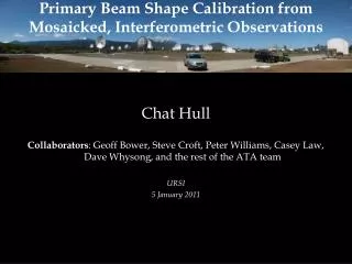
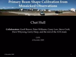
1. Primary Beam Shape Calibration from Mosaicked, Interferometric Observations Chat Hull Collaborators: Geoff Bower, Steve Croft, Peter Williams, Casey Law, Dave Whysong, and the rest of the ATA team UC Berkeley, RAL seminar 8 November 2010

2. Outline • Motivation • Beam-characterization methods • Two-point Gaussian fitting • Chi-squared fitting • Results • Simulation applying method to ATA-350 and SKA

3. The Allen Telescope Array • Centimeter-wave large-number-of-small-dishes (LNSD) interferometer in Hat Creek, CA • Present: ATA-42, 6.1-meter antennas • Wide-band frequency coverage: 0.5 – 11.2 GHz (3-60 cm) • Excellent survey speed (5 deg2 field of view) • Commensal observing with SETI

4. Bad mosaic

5. Good mosaic

6. Motivation • We want to make mosaics • Need to have excellent characterization of the primary beam shape • Primary beam: sensitivity relative to the telescope’s pointing center • Start by characterizing the FWHM of the primary beam using data from ATATS & PiGSS FWHM = 833 pixels Image courtesy of James Gao

7. PiGSSpointings Bower et al., 2010

8. Primary-beam characterization • Primary-beam pattern is an Airy disk • Central portion of the beam is roughly Gaussian • Good approximation down to the ~10% level

9. Primary-beam characterization • In this work we assume our primary beam is a circular Gaussian. • Our goal: to use ATA data to calculate the actual FWHM of the primary beam at the ATATS and PiGSS frequencies.

10. Primary-beam characterization • Canonical value of FWHM:

11. Same source, multiple appearances Pointing 1 Pointing 2 Images courtesy of Steve Croft Can use sources’ multiple appearances to characterize the beam

12. Method 1: Two-point Gaussian solution • We know the flux densities and the distances from the pointing centers • Can calculate the FWHM of a Gaussian connecting this two points

13. Method 1: Two-point Gaussian solution • Analytic solution to the Gaussian between two source appearances: • θ1 , θ2  distances from respective pointing centers • S1 , S2 fluxes in respective pointings

14. Method 1: Two-point Gaussian solution • Solution: • Problems: when S1 ≈ S2and whenθ1 ≈θ2

15. BART ticket across the Bay $3.65 Projected Cost of SKA $2,000,000,000.00 Not being able to use the best part of your data Priceless

16. Method 1: Calculated FWHM values Median primary-beam FWHM values using 2-point method:

17. Method 2: χ2minimization • Find the FWHM value that minimizes • Benefits: • Uses all the data • Can be extended to fit ellipticity, beam angle, etc.

18. Observed flux pairs

19. Corrected flux pairs

20. Method 2: Best-fit FWHM • High values (~21 for ATATS; ~10 for PiGSS) • Due to systematic underestimation of flux density errors, non-circularity of the beam, mismatched sources

21. Method 2: comparison with theory • We see a slightly narrower beam-width • Due to imperfect understanding of ATA antenna response, inadequacy of Gaussian beam model

22. Simulation: applying the χ2 minimization method to future telescopes • As Nant increases, rms noise decreases, and number of detectable sources increases:

23. Simulation: applying the χ2 minimization method to future telescopes • Perform simulation for arrays with NA increasing from 42 to 2688, in powers of 2 • Generate sources across a 12.6 deg2, 7-pointing PiGSS-like field • Use S-2 power-law distribution, down to the rms flux density of the particular array • Add Gaussian noise to flux densities • Note: pointing error not included • “Observe” and match simulated sources • Applyχ2 minimization technique to calculate uncertainty of the FWHM of the primary beam of each array

24. Simulation: results • 42-dish simulation returns FWHM uncertainty of 0.03º • In the absence of systematic errors, the FWHM of the SKA-3000 primary beam could be measured to within 0.02%

25. Conclusions • ATA primary beam has the expected FWHM • Our calculated value: • Chi-squared method is superior to 2-point method • Results are consistent with canonical value (Welch et al.), radio holography (Harp et al.), and the Hex-7 beam characterization technique • Arrived at an answer with zero telescope time • Potential application to other radio telescopes needing simple beam characterization using science data