Basics of Interferometry and Interferometric Calibration

1. Basics of Interferometry and Interferometric Calibration Claire Chandler NRAO/Socorro (with thanks to Rick Perley and George Moellenbrock)

2. Overview • Aperture synthesis • A simple 2-element interferometer • The visibility • The interferometer in practice • Calibration of interferometric data • Baseline-based and telescope-based calibration • Calibration in practice • VLA example • Non-closing errors • Tropospheric phase fluctuations

3. Response of a parabolic antenna Power response of a uniformly-illuminated, circular parabolic antenna (D =25m, n = 1GHz)

4. On-axis incidence Off-axis incidence Origin of the beam pattern • An antenna’s response is a result of coherent phase summation of the electric field at the focus • First null will occur at the angle where one extra wavelength of path is added across the full width of the aperture:q ~ l/D

5. The beam pattern (cont.) • A voltage V(q) is produced at the focus as a result of the electric field • The voltage response pattern is the Fourier Transform of the aperture illumination; for a uniform circle this is J1(x)/x • The power response, P(q) µV2(q) • P(q) is the Fourier Transform of the autocorrelation function of the aperture, and for a uniformly-illuminated circle is the familiar Airy pattern, (J1(x)/x)2 • FWHP = 1.02 l/D • First null at 1.22 l/D

6. Aside: Fourier Transforms • A function or distribution may be described as the infinite sum of sines and cosines with different frequencies (Fourier components), and these two descriptions of the function are equivalent and related by • Where x and s are conjugate variables, e.g.: • Time and frequency, t and 1/t = n • Distance and spatial frequency, l and 1/l = u

7. Some useful FT theorems • Addition • Shift • Convolution • Scaling

8. Output for a filled aperture • Signals at each point in the aperture are brought together in phase at the antenna output (the focus) • Imagine the aperture to be subdivided into N smaller elementary areas; the voltage, V(t), at the output is the sum of the contributions DVi(t) from the N individual aperture elements:

9. Aperture synthesis: basic concept • The radio power measured by a receiver attached to the telescope is proportional to a running time average of the square of the output voltage: • Any measurement with the large filled-aperture telescope can be written as a sum, in which each term depends on contributions from only two of the N aperture elements • Each term áDViDVkñ can be measured with two small antennas, if we place them at locations i and k and measure the average product of their output voltages with a correlation (multiplying) receiver

10. Aperture synthesis: basic concept • If the source emission is unchanging, there is no need to measure all the pairs at one time • One could imagine sequentially combining pairs of signals. For N sub-apertures there will be N(N-1)/2 pairs to combine • Adding together all the terms effectively “synthesizes” one measurement taken with a large filled-aperture telescope • Can synthesize apertures much larger than can be constructed as a filled aperture, giving very good spatial resolution

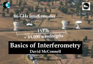
11. s0 a s0 x = u sina q b×s0 u = bcosq u b telescope 2 telescope 1 V1 V2 áV1V2ñ A simple 2-element interferometer • What is the response of the interferometer as a function of position on the sky, l = sina ? • In direction s0(a = 0) the wavefront arriving at telescope 1 has an extra path b×s0= bsinq to travel compared with telescope 2 • The time taken to traverse this path is the geometric delay, tg= b×s0/c • Compensate by inserting a delay in the signal path for telescope 2 equivalent to tg

12. s0 a s0 x = u sina q b×s0 u = bcosq u b telescope 2 telescope 1 V1 V2 áV1V2ñ Response of a 2-element interferometer • At angle a relative to s0 a wavefront has extra path x = usina = ul to travel • Expand to 2D by introducing b orthogonal to a, m = sinb, and v orthogonal to u, so that in this directionthe extra pathy = vm • Write all distances in units of wavelength, x º x/l, u º u/l, etc. so that x and y are now numbers of cycles • Extra path is now ul + vm • V2 = V1 e-2pi(ul+vm)

13. Correlator output • The output from the correlator (the multiplying and time-averaging device) is: • For (l1¹l2, m1¹m2) the above average is zero (assuming mutual incoherence of the sky), so

14. The visibility • Thus the interferometer measures the complex visibility, V, of a source, which is the FT of its intensity distribution on the sky: • u,v are spatial frequencies in the E-W and N-S directions, and are the projected baseline lengths measured in units of wavelength, B/l • l,m are direction cosines relative to a reference position in the E-W and N-S directions • (l=0,m=0) is known as the phase centre

15. A=|V | f Comments on the visibility • This FT relationship is the van Cittert-Zernike theorem, upon which synthesis imaging is based • It means there is an inverse FT relationship that enables us to recover I(l,m) from V (u,v): • The visibility is complex because of the FT • The correlator measures both real and imaginary parts of the visibility to give the amplitude and phase:

16. More comments… • The visibility is a function of the source structure and the interferometer baseline • The visibility is not a function of the absolute position of the telescopes (provided the emission is time-invariant, and is located in the far field) • The visibility is Hermitian: V (-u,-v) = V *(u,v). This is because the sky is real • There is a unique relation between any source brightness distribution and the visibility function • Each observation of the source with a given baseline length, (u,v), provides one measure of the visibility • With many measurements of the visibility as a function of (u,v) we can obtain a reasonable estimate of I(l,m)

17. Some 2D FT pairs Image Visibility amp

18. Some 2D FT pairs Image Visibility amp

19. Some 2D FT pairs Image Visibility amp

20. (u,v) coverage • A single baseline provides one measurement of V (u,v) per time-averaged integration • Build up coverage in the uv-plane by: • having lots of telescopes • moving telescopes around • waiting for the Earth to rotate to provide changing projected baselines, u = bcosq (note: tgchanges continuously too) • some combination of the above Telescope locations: (u,v) coverage for 6 hour track:

21. The measured visibility • Resulting measured visibility: (u,v) coverage VVmeasured ´ = • Note: because the visibility is Hermitian each measurement by the interferometer results in two points in the (u,v) plane, one for baseline 1-2, the other for baseline 2-1, etc.; Earth rotation traces out two arcs per baseline • Recovering I(l,m) from Vmeasured is the topic of the next lecture

22. l/B rad. Source brightness - + - + - + -Fringe Sign Picturing the visibility: fringes • The FT of a single visibility measurement is a sinusoid with spacing l/B between successive peaks, or “fringes” • Build up an image of the sky by summing many such sinusoids (addition theorem) • Scaling theorem shows: • Short baselines have large fringe spacings and measure large-scale structure on the sky • Long baselines have small fringe spacings and measure small-scale structure on the sky

23. The primary beam • The elements of an interferometer have finite size, and so have their own response to the radiation from the sky • This results in an additional factor, A(l,m), to be included in the expression for the correlator output, which is the primary beam or normalized reception pattern of the individual elements • Interferometer actually measures the FT of the sky multiplied by the primary beam response • Need to divide by A(l,m), to recover I(l,m) • The last step in the production of the image

24. Dn n n0 The delay beam • A real interferometer must accept a range of frequencies (amongst other things, there is no power in an infinitesimal bandwidth)! Consider the response of our interferometer over frequency width Dn centred on n0: • At angle a away from the phase centre the excess path for the centre of the band in cycles is u0l • At this point the excess path (in cycles) for the edges of the band, n = n0± Dn/2, is ul = u0l(n/n0)

25. The delay beam (cont.) • Wavefronts are out of phase at the edges of the band compared with the centre where one extra wavelength of path is added across the entire band, or ul-u0l = 0.5 • This occurs where • Now l = sin a » a and fringe spacing qres = 1/u0 • So width of delay beam is • ALMA example: n = 100 GHz, Dn = 8 GHz, D = 12m(qpb = 53²) and qres = 1², Þ qdb~ 12.5² • ALMA will have to divide bandwidth into many channels to avoid loss of sensitivity due to delay beam!

26. The interferometer in practice: the need for calibration • For the ideal interferometer the phase of a point source at the phase centre is zero, because we can correct for the known geometric delay • However, there are other sources of path delay that introduce phase offsets that are telescope-dependent; most importantly at submillimeter wavelengths these are water (vapour and liquid) in the troposphere, and electronics • The raw amplitude of the visibility measured on a given baseline depends on the properties of the two telescopes (gains, pointing, etc.), and must be placed on a physical scale (Jy) • There may be frequency-dependent amplitude and phase responses of the electronics • There may also be baseline-based errors introduced due to averaging in time or frequency • We must observe calibration sources to derive corrections for these effects, to be applied to our program sources

27. Correlation of realistic signals • The signal delivered by telescope i to the correlator is the sum of the voltage due to the source corrupted by a telescope-based complex gain gi(t) = ai(t)eifi(t), where ai(t) is a telescope-based amplitude correction and fi(t) is the telescope-based phase correction, and noise ni(t): • The correlator output is then

28. …realistic signals (cont.) • The noise does not correlate, so the noise term áninj*ñ integrates down to zero • Compare with a single dish, which measures the auto-correlation of the signal: • This is a total power measurement plus noise • Desired signal is not isolated from noise • Noise usually dominates • Single dish calibration strategies dominated by switching schemes to isolate the desired signal

29. Telescope- and baseline-based errors • Write the output from the correlator as where and we have introduced a factor gij(t) to take into account any residual baseline-based gain error • If Gij(t) is slowly-varying this can be written as and we see that the correlator output Vijobs is the true visibility Vij modified by a complex gain factor Gij(t)

30. Contributions to Gij • Gij comprises telescope-based components from: • Ionospheric Faraday rotation (important for cm, not for submm) • Water in the troposphere (important for submm) • Parallactic angle rotation • Telescope voltage pattern response • Polarization leakage • Electronic gains • Bandpass (frequency-dependent amplitudes and phases) • Geometric (delay) compensation (important for VLBI) • Baseline-based errors due to: • Correlated noise (e.g., RFI; important for cm) • Frequency averaging • Time averaging (important for submm because of the troposphere)

31. Solving for Gij • Can separate the various contributions to Gij to give • Initially use estimates (if you have them), or assume Gijn = 1, and solve for the dominant component of the error, assuming we know Vijtrue (note: we observe calibration sources for which we do know Vijtrue) • Iterate on the solutions for Gijn

32. Baseline-based calibration • Since the interferometer makes baseline-based measurements, why not just use the observed (baseline-based) visibilities of calibrator sources to solve for Gij? • We have to know that the calibrator is a point source (i.e., should have f= 0 at the phase centre) or know its structure • If we do not, using baseline-based calibration will absorb structure of the calibrator into the (erroneous) solution for Gij • In general we have to be able to assume that baseline-based effects are astronomical in origin, i.e., tell us about the source visibility (there are some calibrations that are baseline-based; more on these later) • Most gain errors are telescope-based • It is better to solve for N telescope-based quantities than N(N-1)/2 baseline-based quantities (fewer free parameters)

33. Telescope-based calibration: closure relationships • Closure relationships show that telescope-based gain errors do not irretrievably corrupt the information about the source (indeed, in the early days of radio interferometry, and today for optical interferometry, the systems were so phase-unstable that these closure quantities were all that could be measured) • Closure phase (3 baselines); let fij = fi-fj, etc.: • Closure amplitude (4 baselines): fi+Dfi fj+Dfj fk+Dfk

34. Calibration in practice • Observe nearby point sources against which calibration can be solved, and transfer solutions to target observations • Choose appropriate calibrators; usually strong point sources because we can predict their visibilities • Choose appropriate timescales for calibration • Typically need calibrators for: • Absolute flux density (constant radio source, planet) • Nearby point source to track complex gain • Nearby point source for pointing calibration • Strong source for bandpass measurement • Source with known polarization properties for instrumental polarization calibration

35. VLA example • Science: • HI observations of the galaxy NGC2403 • Sources: • Target source: NGC2403 • Near-target calibrator: 0841+708 (8 deg from target; unknown flux density, assume 1 Jy initially) • Flux density calibrators: 3C48 (15.88 Jy), 3C147 (21.95 Jy), 3C286 (14.73 Jy) • Signals: • RR correlation, total intensity • 1419.79 MHz (HI), one 3.125 MHz channel • (continuum version of a spectral line observation)

36. Observing sequence

37. UV-coverages

38. Views of the raw data

39. Uncalibrated images

40. Gain errors are telescope-based

41. The telescope-based calibration solution - I • Solve for telescope-based gain factors on 600s timescale (1 solution per scan on near-target calibrator, 2 solutions per scan on flux-density calibrators): • Bootstrap flux density scale by scaling mean gain amplitudes of near-target (nt) calibrator (assumed 1Jy above) according to mean gain amplitudes of flux density (fd) calibrators:

42. The telescope-based calibration solution - II

43. Calibrated calibrator phases - I

44. Calibrated calibrator phases - II

45. Calibrated visibilities

46. Calibrated images

47. Evaluating the calibration • Are solutions continuous? • Noise-like solutions are just that—noise • Discontinuities indicate instrumental glitches • Any additional editing required? • Are calibrator data fully described by antenna-based effects? • Phase and amplitude closure errors are the baseline-based residuals • Are calibrators sufficiently point-like? If not, self-calibrate • Any evidence of unsampled variation? Is interpolation of solutions appropriate? • Reduce calibration timescale, if SNR (and data) permits • Evidence of gain errors in your final image? • Phase errors give asymmetric features in the image • Amplitude errors give symmetric features in the image

48. Typical calibration sequence, spectral line • Preliminary solve for G on bandpass calibrator: • Solve for bandpass on bandpass calibrator: • Solve for G (using B) on gain calibrator: • Flux density scaling: • Correct the data: • Image!

49. Non-closing errors • Baseline-based errors are non-closing errors (they do not obey the closure relationships) • The three main sources of non-closing errors arise from • Source structure! • Frequency averaging • Time averaging • Frequency averaging: • Instrument has a telescope-based bandpass response as a function of frequency • If all telescopes have the same response then averaging in frequency will preserve the closure relationships • Different bandpass responses will introduce baseline-based gain errors (e.g., VLA-EVLA baselines)

50. Non-closing bandpass errors • Solutions: • Design your instrument to match bandpasses as closely as possible • Divide the bandpass into many channels, so that the closure relationships are obeyed on a per-channel basis • Apply a baseline-based calibration • BUT BEWARE OF FREQUENCY-DEPENDENT STRUCTURE IN THE CALIBRATION SOURCE