Download
1 / 20
200 likes | 292 Views
Explore beam characterization and Gaussian solutions from mosaicked observations with ATA-42. Analyze FWHM values, observed flux pairs, and beam holography for precise data representation. Future work includes PiGSS data comparison and statistical treatment.

E N D
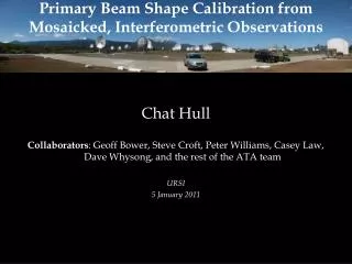
Primary Beam Shape Calibration from Mosaicked Observations Chat Hull Collaborators: Geoff Bower, Peter Williams, Casey Law, Steve Croft, Dave Whysong, Gerry Harp, and the rest of the ATA team GSPS 4 December 2009
The Allen Telescope Array • Centimeter-wave LNSD interferometer in Hat Creek, CA • Commensal observing with SETI • Wide-band frequency coverage: 0.5 – 11.2 GHz (3-60 cm) • Excellent survey speed (5 deg2 FOV) • Present: ATA-42, 6.1-meter antennas • Future: ATA-350 – greater sensitivity
Beam characterization • Beam: sensitivity relative to the telescope’s pointing center • Beam pattern is a sinc function (Airy disk – response of a parabolic antenna) • Central portion of the beam is roughly Gaussian • Good approximation out to the ~10% level • By that point, other effects dominate (sidelobes, reflections)
Motivation • Want to make mosaics • Need to have excellent characterization of the primary beam shape • My aim: characterize it! • Using archival data from ATATS • Start with FWHM • Canonical value:
Same source, multiple appearances Pointing 1 Pointing 2 Images courtesy of Steve Croft • Can use multiple matches of many sources to characterize the beam
Two-point Gaussian solution • Analytic solution to the Gaussian between two source appearances: • r1 , r2 distances from respective pointing centers • S1 , S2 fluxes in respective pointings
Two-point Gaussian solution • Solution: • Problems: when S1 ≈ S2 and when r1 ≈ r2
Problematic pairs Observed flux ratios
Problematic pairs Distance ratios
BART ticket across the Bay $3.65 2012 projection of UC Berkeley undergraduate fees $465,700.31 Not being able to use the best part of your data Priceless
Observed flux pairs Untrimmed, uncorrected
Observed flux pairs Trimmed, uncorrected
Corrected flux pairs Untrimmed, corrected
Corrected flux pairs Trimmed, corrected
Other beam characterizations • Hex-7 results • FWHM values close to canonical value • Beam holography • Slightly larger value
Future work • PiGSS data • Constrain beam angle and ellipticity • Will have to contend with transformation from RA/Dec to Az/El • Compare these synthesized results with Gerry’s antenna-by-antenna results • Tweak the Gaussian approximation when solving for FWHM • Give a more rigorous statistical treatment to the data (MLE?)
Conclusions • Beam has the expected FWHM! • Our value: • Telescope is producing the data we expect • Arrived at an answer with zero telescope time • Potential application to other radio telescopes needing simple beam characterization