Combinational Logic
Chapter 4. Combinational Logic. 4.1 Introduction. Logic circuits for digital systems may be. . combinational or sequential. A combinational circuit consists of logic gates. . whose outputs at any time are determined. from only the present combination of inputs. 2.

Combinational Logic
E N D
Presentation Transcript
Chapter 4 Combinational Logic
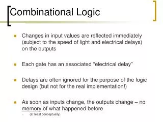
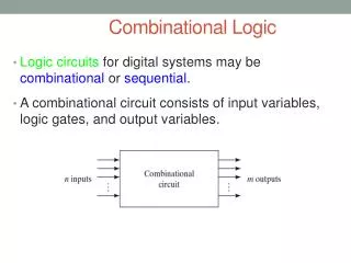
4.1 Introduction Logic circuits for digital systems may be combinational or sequential. A combinational circuit consists of logic gates whose outputs at any time are determined from only the present combination of inputs. 2
4.2 Combinational Circuits Logic circuits for digital system Sequential circuits contain memory elements the outputs are a function of the current inputs and the state of the memory elements the outputs also depend on past inputs 3
A combinational circuits n 2 possible combinations of input values Combinational circuits n input m output Combinatixnal variables variables xoxic Circuit Specific functions Adders, subtractors, comparators, decoders, encoders, and multiplexers 4
4-3 Analysis Procedure A combinational circuit make sure that it is combinational not sequential No feedback path derive its Boolean functions (truth table) design verification
A straight-forward procedure F = AB+AC+BC 2 T = A+B+C = AxB+C 1 1 T = ABC 2 T = F2'T1 3 F = T3+T2 1 6
F = T +T = F 'T +ABC 1 3 2 2 1 = (AB+AC+BC)'(A+B+C)+ABC = (A'+B')(A'+C“)(B'+C')(A+B+C)+ABC = (A'+B'C')(AB'+AC'+BC'+B'C)+ABC = A'BC'+A'B‘C+AB‘C'+ABC 7
The truth table 8
4-4 Design Procedure The design procedure of combinational circuits State the problem (system spec.) determine the inputs and outputs the input and output variables are assigned symbols derive the truth table ed b x derive the simplifi erive the simplified Bool oolean functions xan functionx draw the logic diagram and verify the correctness 9
Functional description Boolean function HDL (Hardware description language) Verilog HDL VHDL Schematic entry Logic minimization number of gates number of inputs to a gate Propagation delay number of interconnection limitations of the driving capaeilities 10
Cdde conversion example BCD to excess-3 code The truth table 11
The maps 12
The simplified functions z = D' y = CD +C'D‘ x = B'C + B‘D+BC'D' w = A+BC+BD Another i mplementation z = D' y = CD +C'D' = CD + (C+D)' x = B'C + B'D+BC'D‘ = B'(C+D) +B(C+D)' w = A+BC+BD 13
The logic diagram 14
4-5 Binary Adder-Subtractor Half adder 0 + 0 = 0 ; 0 + 1 = 1 ; 1 + 0 = 1 ; 1 + 1 = 10 two input variables: x, y two output variables: C (carry), S (sum) truth table 15
S = x'y+xy' C = xy the flexibility for implementation S=xÅy S = (x+y)(x'+y') S‘= xy+x'y' S = (C+x'y')' C = xy = (x'+y')x 16
CS 151 Functional Block: Full-Adder Z 0 0 0 0 X 0 0 1 1 + Y + 0 + 1 + 0 + 1 C S 0 0 0 1 0 1 1 0 Z 1 1 1 1 X 0 0 1 1 + Y + 0 + 1 + 0 + 1 C S 0 1 1 0 1 0 1 1 A full adder is similar to a half adder, but includes a carry-in bit from lower stages. Like the half-adder, it computes a sum bit, S and a carry bit, C. For a carry-in (Z) of 0, it is the same as the half-adder: For a carry- in(Z) of 1:
Full-Adder The arithmetic sum of three input bits three input bits x, y: two significant bits z: the carry bit from the previous lower significant bit Two output bits: C, S 18
S = x'y'z+x'yz'+ xy'z'+xyz C = xy + xz + yz S = zÅ (xÅy) = z'(xy'+x‘y)+z(xy'+x'y)' = z‘xy'+z'x'y+z(xy+x‘y') = xy'z'+x'yz'+xyz+x'y'z C = z(xy'+x'y)+xy = xy'z+x'yz+ xy 20
Binary adder 21
Binary adder subtractor A-B = A+(2’s complement of B) 4-bit Adder-subtractor M=0, A+B; M=1, A+B’+1 26
Overflow The storage is limited Add two positive numbers and obtain a negative number Add two negative numbers and obtain a positive number V = 0, no overflow; V = 1, overflow Example: 27
4-6 Decimal Adder Add two BCD's 9 inputs: two BCD's and one carry-in 5 outputs: one BCD and one carry-out Design approaches A truth table with 2^9 entries use uinary full Adders the sum <= 9 + 9 + 1 = 19 binary to BCD 25
Modifications are needed if the sum > 9 C = 1 K = 1 Z Z = 1 8 4 Z Z = 1 8 2 mo mo x d ification: ification: - - (10) (10) or +6 or +6 d d C = K +Z Z + Z Z 8 4 8 2 27
Block diagram 28
Binary Multiplier Partial products – AND operations fig. 4.15 Two-bit by two-bit binary multiplier. 29
4-bit by 3-bit binary multiplier Fig. 4.16 Four-bit by three-bit binary multiplier. Digital Circuits 30
4-9 Decoder A n-to-m decoder n a binary code of n bits = 2 distinct information n n input variables; up to 2 output lines only one output can be active (high) at any time 31
An implementation Fig. 4.18 Three-to-eight-line decoder. 38 Digital Circuits 32
Combinational logic implementation each output = a minterm use a decoder and an external OR gate to implement any Boolean function of n input variables 33
Demultiplexers a decoder with an enable input receive information in a single line and transmits n it in one of 2 possible output lines Fig. 4.19 Two-to-four-line decoder with enable input 34
Decoder Examples • 3-to-8-Line Decoder: example: Binary-to-octal conversion. D0 = m0 = A2’A1’A0’ D1= m1 = A2’A1’A0 …etc
Expansion two 3-to-8 decoder: a 4-to-16 deocder Fig. 4.20 4 16 decoder constructed with two 3 x 8 decoders a 5-to-32 decoder? 36
Decoder Expansion - Example 2 A0 A1 A2 3-8-line Decoder D0 – D7 E 3-8-line Decoder D8 – D15 A3 A4 E 2-4-line Decoder 3-8-line Decoder D16 – D23 E 3-8-line Decoder D24 – D31 E Construct a 5-to-32-line decoder using four 3-8-line decoders with enable inputs and a 2-to-4-line decoder. CS 151
Combination Logic Implementation each output = a minterm use a decoder and an external OR gate to implement any Boolean function of n input variables A full-adder S(x,y,z)=S(1,2,4,7) C(x,y,z)= C(x,y,z)= S S (3,5,6,7) (3,5,6,7) Fig. 4.21 Implementation of a full adder with 1 decoder 38
two possible approaches using decoder OR(minterms of F): k inputs n NOR(minterms of F'): 2 - k inputs In general, it is not a practical implementation 39
4-10 Encoders The inverse function of decoder a decoder z = D + D + D + D 1 3 5 7 The encoder can be implemented y = D + D + D + D 2 3 6 7 with three OR gates. x = D + D + D + D 4 5 6 7 40
An implementation limitations illegal input: e.g. D =D x1 3 6 The output = 111 (¹3 and ¹6) 41
Priority Encoder resolve the ambiguity of illegal inputs only one of the input is encoded D has the highest priority 3 D has the lowest priority 0 X: don't-care conditions V: valid output indicator 42
■ The maps for simplifying outputs x and y fig. 4.22 Maps for a priority encoder 43
■ Implementation of priority x = D + D Fig. 4.23 2 3 Four-input priority encoder x = ¢ D + D D 3 1 2 V = x + D + D + D 0 1 2 3 44
4-11 Multiplexers select binary information from one of many input lines and direct it to a single output line n 2 input lines, n selection lines and one output line e.g.: 2-to-1-line multiplexer Fig. 4.24 Two-to-one-line multiplexer 45
4-to-1-line multiplexer Fig. 4.25 Four-to-one-line multiplexer 46
Note n n-to- 2 decoder n add the 2 input lines to each AND gate OR(all AND gates) an enable input (an option) 47
Fig. 4.26 Quadruple two-to-one-line multiplexer 48
Boolean function implementation MUX: a decoders an OR gate n 2 -to-1 MUX can implement any Boolean function of n input variable a better solution: implement any Boolean function of n+1 input variable n of these variables: the selection lines the remaining variable: the inputs 49
an example: F(A,B,C) = S(1,2,6,7) Fig. 4.27 Implementing a Bolxean function with a multiplexer 50