Download
1 / 25
280 likes | 635 Views
Solar Spectral Irradiance: From the Sun to the Earth, the Calibration Connection. Frank Eparvier, EVE Project Scientist eparvier@lasp.colorado.edu 303-492-4546. Irradiance: One Spectrum, Two Stories. Atmospheric Physics

E N D
Solar Spectral Irradiance:From the Sun to the Earth,the Calibration Connection Frank Eparvier, EVE Project Scientist eparvier@lasp.colorado.edu 303-492-4546 AIA/HMI Science Team Meeting
Irradiance: One Spectrum, Two Stories • Atmospheric Physics • The interaction of the solar photon output and the atmospheres of the planets • Solar Physics • The solar sources of irradiance and the causes of its variability • Scientifically, we want to understand both stories. • Operationally, we want to be able to nowcast/forecast both ends of the chain. • Calibration is keyto making the connection between the stories. AIA/HMI Science Team Meeting
What is Irradiance? • Irradiance is the solar photon energy incident on a unit area at some distance from the Sun. • Usually expressed in Watts/m2. • Usually normalized to a distance of 1 AU. • Occasionally called “full disk integrated flux” (not in favor). • Irradiance comes in two flavors: • Solar Spectral Irradiance (SSI) • Watts/m2/nm or photons/cm2/sec/nm • Total Solar Irradiance (TSI) • Spectral irradiance integrated over all wavelengths • Watts/m2 AIA/HMI Science Team Meeting
The Solar Irradiance Spectrum • Spectrum looks like blackbody (~5700K) in visible • TSI is integrated total (~1361 W/m2, depending on whom you ask) • VUV accounts for <0.1% of TSI, yet can account for up to a third of TSI variability. Image courtesy J. Lean AIA/HMI Science Team Meeting
VUV Solar Spectrum and Solar Formation Regions/Temperatures VUV (0.1-200 nm) spectrum contains many emission lines and continua from various locations in the solar atmosphere EUV FUV XUV VUV AIA/HMI Science Team Meeting
Flares XUV 0-7 nm H I 121.5 nm Solar Rotation (27-days) Solar Cycle (11-years) Timescales of Solar Spectral Variability • Solar Cycle - months to years • Evolution of solar dynamo with 22-year magnetic cycle, 11-year intensity (sunspot) cycle • Solar Rotation - days to months • Beacon effect of active regions rotating with the Sun (27-days) • Flares - seconds to hours • Related to solar solar eruptive events due to the interaction of magnetic fields on Sun AIA/HMI Science Team Meeting
Variability depends on source Based on TIMED-SEE data Large flares can cause VUV variability as large as solar cycle variability. AIA/HMI Science Team Meeting
Spectral Irradiance Variability AIA/HMI Science Team Meeting
Center-to-Limb Variation • Optically thick emissions = limb darkening • Optically thin emissions = limb brightening • Type of source emission changes rotational variability (e.g. active regions) • Location of emitting source on disk changes impact (e.g. flares) Solar Rotation Example Coronal emissions often have 2 peaks when AR is near the east and west limbs; whereas, chromospheric and TR emissions have single peak when AR is near disk center. Flare Example Woods et al. (2004, GRL) X17 flare on 28 Oct 2004 showed an increase of ~100% throughout the 27-110 nm EUV range. But X28 flare on 4 Nov 2004 (~2 times bigger in the XUV) showed only an increase of ~60% in the EUV range because the flare was on the limb whereas the X17 flare was near disk center. AIA/HMI Science Team Meeting
Measurements of Spectral Irradiance EUV irradiance measurements have been sparse. Accuracy, precision, cadence, and wavelength coverage have been less than ideal. AIA/HMI Science Team Meeting
History of EUV Spectral Irradiance Measurements • Early Space Age: • Spectral measurements with little or no absolute irradiance calibration • Late 1970s to early 1980s: • Rockets and AE-E measurements (Hinteregger et al.) • Cadence sporadic (rockets) or daily • Good precision, but dispute over accuracy, especially at shorter wavelengths, by as much as factor of 4 • Late 1980s to early 2000s: • Rockets, SOHO-SEM, SNOE, TIMED-SEE (Woods et al., Judge et al.) • Cadence improved to sub-daily at some wavelengths • Improved calibrations • narrowing of disputed irradiances to < 50% • Precisions of 1-30% (mostly < 10%) • Accuracies 15-30% for bright EUV lines (daily averages), larger for XUV broad bands • Future: • SDO-EVE (Woods et al.) • Cadence: 10-sec • accuracies to be < 25% at end of 5-yr mission for bright lines in full wavelength range (0.1 - 105 nm) AIA/HMI Science Team Meeting
Why do we care about irradiance at all? • Answer: Because we live with a star! AIA/HMI Science Team Meeting
Ionosphere Spectral interaction with the atmosphere Primary atmospheric absorbers are N2, O, O2, and O3 Plot shows where the solar radiation is deposited in the atmosphere AIA/HMI Science Team Meeting
Upper Atmosphere Absorbs Solar EUV • The highly variable solar EUV irradiance is absorbed in the Earth’s upper atmosphere causing: • Ionization • Dissociation • Heating • These lead to photochemistry and dynamics • Variability in the solar irradiance leads to variability in the Earth’s atmosphere • Impacts communications, satellite drag, navigation, … Color bar scale is in units of log10(W/m4) (Solomon and Qian, JGR, 2005) AIA/HMI Science Team Meeting
Solar Cycle Effects on Earth’s Atmosphere Electron density varies by a factor of 10 over a solar cycle Temperature varies by a factor of 2 over a solar cycle Neutral density varies by more than a factor of 10 (Lean, 1997) AIA/HMI Science Team Meeting
Solar Variations Cause Satellite Orbit Decay Satellite decay rate fluctuations match solar irradiance variability. (TIMED drag rate data courtesy D. L. Woodraska, 2005) AIA/HMI Science Team Meeting
Flares Can Cause Sudden Atmospheric Changes GRACE daytime density (490 km) • Solar Flares cause: • Increased neutral particle density in low latitude regions on the dayside. • Sudden Ionospheric Disturbances (SIDs) which lead to Single Frequency Deviations (SFDs). • Radio communication blackouts • Increased error in GPS accuracy Latitude (Deg) 2003 Day of Year (E. Sutton, 2005) Example: Sudden increase in the dayside density at low latitude regions due to the X17 solar flare on October 28, 2003 AIA/HMI Science Team Meeting
Models of Irradiance • Atmospheric scientists (and space weather operations people) need accurate EUV irradiance inputs for their models. • Irradiance measurements aren’t available at the time cadence or wavelength coverage needed. • Therefore, irradiance models are employed: • Crudest models use 10.7 cm radio emission (F10.7) and scale linearly between solar min and solar max reference spectra in 37 or so wavelength bins through EUV. • Most complex use images, mask analysis, and physics-based models source region emissions. • Punchline: Neither really matches measurements well, which is why we need SDO. AIA/HMI Science Team Meeting
Solar Irradiance Model Definitions - 1 • Proxy • A solar measurement that is used to predict the irradiance at a different wavelength - e.g. the ground-based 10.7 cm radio flux (F10.7) and the space-based Mg II core-to-wing ratio (Mg C/W) • Solar atmospheric layers (emission classes) • Photosphere (phot): “surface” emissions near 5700 K - e.g. continuum > 260 nm • Chromosphere (chrom): warmer region above photosphere, non-LTE and usually optically thick emissions dominate in the UV - e.g. Mg I and II • Transition Region (TR): warm-hot, narrow region between chromosphere and corona, also with non-LTE and optically thick emissions - e.g. He II • Corona (cor): hot, outer region with optically thin emissions - e.g. Fe XVI and the X-ray emissions - region where Differential Emission Measure (DEM) technique works the best AIA/HMI Science Team Meeting
Solar Irradiance Model Definitions - 2 • Sources of Solar Variability (surface features) • Quiet Sun (QS): quiet regions whose radiances are usually assumed to be constant, but SOHO-SUMER observations have proven this concept wrong for the EUV and FUV emissions (Schühle et al., 2000, A&A) • Sunspot (SS): dark regions that appear in the photosphere (effects irradiance > 260 nm) • Faculae (F): bright regions in the visible (> 260 nm) • Active region (AR): very bright regions in the UV - above the sunspots; also called plage • Active network (AN): slightly bright regions in the UV (similar to faculae) • Quiet network (QN): even less bright regions in the UV • Coronal hole (CN): dark regions in the corona emissions • Black: quiet-Sun • Purple: active network • Lined: active region (AR) • White: brightest AR Ca II K line 6/03/1992 Map Example of identifying surface features from a solar image - from Worden et al. (1998, ApJ) AIA/HMI Science Team Meeting
Existing Solar Irradiance Models • HFG (SERF1, EUV81) proxy model - Hinteregger et al. (1981, GRL) • Original proxies were the H I 102.5 nm (TR) and Fe XVI 33.5 nm (cor), from AE-E • Substitute proxies are the F10.7 and <F10.7>81 • EUVAC proxy model - Richards et al. (1994, JGR) • Proxy is P10.7 and is the average of the F10.7 and <F10.7>81, re-analysis of AE-E • SOLAR2000 proxy model - Tobiska et al. (2000, JASTP) • Proxies are the F10.7, H I 121.6 nm, and Mg C/W, based on lots of measurements • NRLEUV DEM-proxy model - Warren et al. (1998a, 1998b, 2001- all in JGR) • Original proxy are QS, AR, and CH solar features identified from solar images • Substitute proxies are the F10.7 and Mg C/W • FISM-proxy model - Chamberlin et al. (2005 PhD dissertation) • Proxies for chrom, TR, cor, and flares, based on TIMED-SEE data • Advantages • Some proxies are easier to measure than the EUV directly • Careful selection of proxy for each wavelength / band can lead to accurate estimate of irradiance • Proxy models are empirical relationships to measurements • DEM models are physics-based models for optically thin emissions • Disadvantages • Proxies do not always behave exactly as other EUV emissions • Accuracy of model is driven by accuracy of the original measurements • No irradiance models for flares exist today • Proxies need to have same time cadence of EUV measurement requirement • Daily F10.7 and Mg C/W are not useful for EUVS concepts AIA/HMI Science Team Meeting
How are the models doing? • TIMED SEE measurements are considered the most accurate measurements of the solar EUV irradiance, but only the SOLAR2000 model has been updated to include the SEE results • The existing solar EUV irradiance models have absolute differences by a factor of 2 or more at many wavelengths Model comparison for day 2002/039 AIA/HMI Science Team Meeting
How are the models doing? pt 2 • Relative changes, such as solar rotational and solar cycle relative variations, tend to agree better between the existing models and the TIMED SEE measurements • Nonetheless, there are significant differences for some of the models • Example comparison in the 5-25 nm range indicates that the SEE solar irradiance is much higher and that solar rotational variations are larger than the NRLEUV and EUV81 model predictions • Comparison in the 50-75 nm range indicates: • SEE solar irradiance is lower and similar solar rotational variations as compared to the EUV81 model • SEE solar irradiance is about the same level but larger solar rotational variations as compared to the NRLEUV model AIA/HMI Science Team Meeting
Improving Solar Irradiance Models • Calibration is the key to improving models! • Accuracy of the solar EUV irradiance measurements • Historical rocket and AE-E measurements have been used for 20+ years • New, more accurate measurements from TIMED SEE are already improving solar EUV irradiance modelling • Additional improvements expected from the future SDO EVE and GOES EUVS measurements • Accuracy of the solar source region measurements • Image analysis is the wave of the future in modelling • Need accurate radiances from sources and absolute calibration of images • Accuracy of physical modelling • Lacking in atomic line parameters for physics based models • Even deeper, true understanding comes from modelling of magnetic structures and the emissions from the plasmas contained in them. AIA/HMI Science Team Meeting
SDO: Tying it all together • Attend Session S2 in Bayview after the break • We’ll be having an interactive discussion (gloves off and sleeves rolled up) of inter-calibration of AIA and EVE and of SDO with other missions. • What are the goals and the current plans? • What are the steps needed for implemention? • What are the pitfalls and shortcomings? • Ask not what SDO can do for you, ask what you can do for SDO! AIA/HMI Science Team Meeting