Download

1 / 32
320 likes | 477 Views
Power 14 Goodness of Fit & Contingency Tables. Outline. I. Parting Shots On the Linear Probability Model II. Goodness of Fit & Chi Square III.Contingency Tables. The Vision Thing. Discriminating BetweenTwo Populations Decision Theory and the Regression Line. education. Players. Mean

E N D
Outline • I. Parting Shots On the Linear Probability Model • II. Goodness of Fit & Chi Square • III.Contingency Tables
The Vision Thing • Discriminating BetweenTwo Populations • Decision Theory and the Regression Line
education Players Mean Educ Players Discriminating line Non-players Mean educ. non income mean income non Mean income Players mx = a, sx2 > sy2 my = b rx, y > 0
Expected Costs of Misclassification • E CMC = C(n/p)*P(n/p)*P(p) + C(p/n)*P(n/p)*P(p) • where P(n) = 23/100 • Suppose C(n/p) = C(p/n) • then E CMC = C*P(n/p)*3/4 + C*P(p/n)*1/4 • And the two costs of misclassification will be balanced if P(p/n) =3/4 = Bern
The Regression Line-Discriminant Function • Bern = 3/4 • Bern = c + b1 *educ + b2 *income • Bern = 3/4 = 1.39 - 0.0216*educ -0.0105* income, or • 0.0216*educ =0.64 - 0.0105*income • Educ = 29.63 - 0.486*income, • the regression line
Lottery: Players and Non-Players Vs. Education & Income 25 Discriminant Function or Decision Rule: Bern = ¾ = 1.39 – 0.0216*education – 0.0105*income 20 15 Education (Years) 10 Legend: Non-Players Players 5 Mean-Players Mean- Nonplayers 0 0 10 20 30 40 50 60 70 80 90 100 Income ($000)
II. Goodness of Fit & Chi Square • Rolling a Fair Die • The Multinomial Distribution • Experiment: 600 Tosses
The Expected Frequencies & Empirical Frequencies Empirical Frequency
Hypothesis Test • Null H0: Distribution is Multinomial • Statistic: (Oi - Ei)2/Ei, : observed minus expected squared divided by expected • Set Type I Error @ 5% for example • Distribution of Statistic is Chi Square One Throw, side one comes up: multinomial distribution P(n1 =1, n2 =0, n3 =0, n4 =0, n5 =0, n6 =0) = n!/ P(n1 =1, n2 =0, n3 =0, n4 =0, n5 =0, n6 =0)= 1!/1!0!0!0!0!0!(1/6)1(1/6)0 (1/6)0 (1/6)0 (1/6)0 (1/6)0
5 % 11.07 Chi Square Density for 5 degrees of freedom
Contingency Table Analysis • Tests for Association Vs. Independence For Qualitative Variables
Does Consumer Knowledge Affect Purchases? Frost Free Refrigerators Use More Electricity
Joint Disribution Under Independence f(x,y) = f(x)*f(y)
Contribution to Chi Square: (observed-Expected)2/Expected Upper Left Cell: (314-324)2/324 = 100/324 =0.31 Chi Sqare = 0.31 + 0.93 + 0.46 +1.39 = 3.09 (m-1)*(n-1) = 1*1=1 degrees of freedom
5% 5.02
Using Goodness of Fit to Choose Between Competing Proabaility Models • Men on base when a home run is hit
Conjecture • Distribution is binomial
Average # of men on base Sum of products = n*p = 0.298+0.250+0.081 = 0.63
Using the binomialk=men on base, n=# of trials • P(k=0) = [3!/0!3!] (0.21)0(0.79)3 = 0.493 • P(k=1) = [3!/1!2!] (0.21)1(0.79)2 = 0.393 • P(k=2) = [3!/2!1!] (0.21)2(0.79)1 = 0.105 • P(k=3) = [3!/3!0!] (0.21)3(0.79)0 = 0.009
Chi Square, 3 degrees of freedom 5% 7.81
Conjecture: Poisson where m=np = 0.63 • P(k=3) = 1- P(k=2)-P(k=1)-P(k=0) • P(k=0) = e-m mk /k! = e-0.63 (0.63)0/0! = 0.5326 • P(k=1) = e-m mk /k! = e-0.63 (0.63)1/1! = 0.3355 • P(k=2) = e-m mk /k! = e-0.63 (0.63)2/2! = 0.1057