Download
1 / 45
480 likes | 959 Views
Elastic Buckling Behavior of Beams. CE579 - Structural Stability and Design. ELASTIC BUCKLING OF BEAMS. Going back to the original three second-order differential equations:. 1. (M TY +M BY ). (M TX +M BX ). 2. 3. ELASTIC BUCKLING OF BEAMS.

E N D
Elastic Buckling Behavior of Beams CE579 - Structural Stability and Design
ELASTIC BUCKLING OF BEAMS • Going back to the original three second-order differential equations: 1 (MTY+MBY) (MTX+MBX) 2 3
ELASTIC BUCKLING OF BEAMS • Consider the case of a beam subjected to uniaxial bending only: • because most steel structures have beams in uniaxial bending • Beams under biaxial bending do not undergo elastic buckling • P=0; MTY=MBY=0 • The three equations simplify to: • Equation (1) is an uncoupled differential equation describing in-plane bending behavior caused by MTX and MBX 1 (-f) 2 3
ELASTIC BUCKLING OF BEAMS • Equations (2) and (3) are coupled equations in u and f – that describe the lateral bending and torsional behavior of the beam. In fact they define the lateral torsional buckling of the beam. • The beam must satisfy all three equations (1, 2, and 3). Hence, beam in-plane bending will occur UNTIL the lateral torsional buckling moment is reached, when it will take over. • Consider the case of uniform moment (Mo) causing compression in the top flange. This will mean that • -MBX = MTX = Mo
Uniform Moment Case • For this case, the differential equations (2 and 3) will become:
ELASTIC BUCKLING OF BEAMS • Assume simply supported boundary conditions for the beam:
Uniform Moment Case • The critical moment for the uniform moment case is given by the simple equations shown below. • The AISC code massages these equations into different forms, which just look different. Fundamentally the equations are the same. • The critical moment for a span with distance Lb between lateral - torsional braces. • Py is the column buckling load about the minor axis. • Pis the column buckling load about the torsional z- axis.
Non-uniform moment • The only case for which the differential equations can be solved analytically is the uniform moment. • For almost all other cases, we will have to resort to numerical methods to solve the differential equations. • Of course, you can also solve the uniform moment case using numerical methods
What numerical method to use • What we have is a problem where the governing differential equations are known. • The solution and some of its derivatives are known at the boundary. • This is an ordinary differential equation and a boundary value problem. • We will solve it using the finite difference method. • The FDM converts the differential equation into algebraic equations. • Develop an FDM mesh or grid (as it is more correctly called) in the structure. • Write the algebraic form of the d.e. at each point within the grid. • Write the algebraic form of the boundary conditions. • Solve all the algebraic equations simultaneously.
Finite Difference Method f Forward difference Backward difference f’(x) Central difference f(x) f(x+h) f(x-h) x h h
Finite Difference Method h i-2 1 2 i-1 i i+1 n 3 i+2 • The central difference equations are better than the forward or backward difference because the error will be of the order of h-square rather than h. • Similar equations can be derived for higher order derivatives of the function f(x). • If the domain x is divided into several equal parts, each of length h. • At each of the ‘nodes’ or ‘section points’ or ‘domain points’ the differential equations are still valid.
Finite Difference Method • Central difference approximations for higher order derivatives:
FDM - Beam on Elastic Foundation 1 3 4 6 2 5 h =0.2 l • Consider an interesting problemn --> beam on elastic foundation • Convert the problem into a finite difference problem. w(x)=w Fixed end Pin support K=elastic fdn. x L Discrete form of differential equation
FDM - Beam on Elastic Foundation 0 7 1 3 4 6 2 5 h =0.2 l Need two imaginary nodes that lie within the boundary Hmm…. These are needed to only solve the problem They don’t mean anything.
FDM - Beam on Elastic Foundation • Lets consider the boundary conditions:
FDM - Beam on Elastic Foundation • Substituting the boundary conditions: Let a = kl4/625EI
FDM - Column Euler Buckling 5 P 0 1 2 4 3 6 x w P Buckling problem: Find axial load P for which the nontrivial Solution exists. x L Finite difference solution. Consider case Where w=0, and there are 5 stations h=0.25L
FDM - Column Euler Buckling • Final Equations
FDM - Euler Buckling Problem • [A]{y}+[B]{y}={0} • How to find P? Solve the eigenvalue problem. • Standard Eigenvalue Problem • [A]{y}={y} • Where, = eigenvalue and {y} = eigenvector • Can be simplified to [A-I]{y}={0} • Nontrivial solution for {y} exists if and only if | A-I|=0 • One way to solve the problem is to obtain the characteristic polynomial from expanding | A-I|=0 • Solving the polynomial will give the value of • Substitute the value of to get the eigenvector {y} • This is not the best way to solve the problem, and will not work for more than 4or 5th order polynomial
FDM - Euler Buckling Problem • For solving Buckling Eigenvalue Problem • [A]{y} + [B]{y}={0} • [A+ B]{y}={0} • Therefore, det |A+ B|=0 can be used to solve for
FDM - Euler Buckling Problem 5 P 0 1 2 4 3 6 x • 11% error in solution from FDM • {y}= {0.4184 1.0 0.8896}T
FDM Euler Buckling Problem • Inverse Power Method: Numerical Technique to Find Least Dominant Eigenvalue and its Eigenvector • Based on an initial guess for eigenvector and iterations • Algorithm • 1) Compute [E]=-[A]-1[B] • 2) Assume initial eigenvector guess {y}0 • 3) Set iteration counter i=0 • 4) Solve for new eigenvector {y}i+1=[E]{y}i • 5) Normalize new eigenvector {y}i+1={y}i+1/max(yji+1) • 6) Calculate eigenvalue = 1/max(yji+1) • 7) Evaluate convergence: i+1-i < tol • 8) If no convergence, then go to step 4 • 9) If yes convergence, then = i+1 and {y}= {y}i+1
Beams with Non-Uniform Loading • Let Mocr be the lateral-torsional buckling moment for the case of uniform moment. • If the applied moments are non-uniform (but varying linearly, i.e., there are no loads along the length) • Numerically solve the differential equation using FDM and the Inverse Iteration process for eigenvalues • Alternately, researchers have already done these numerical solution for a variety of linear moment diagrams • The results from the numerical analyses were used to develop a simple equation that was calibrated to give reasonable results.
Beams with Non-uniform Loading • Salvadori in the 1970s developed the equation below based on the regression analysis of numerical results with a simple equation • Mcr = Cb Mocr • Critical moment for non-uniform loading = Cb x critical moment for uniform moment.
Beams with Non-Uniform Loading • In case that the moment diagram is not linear over the length of the beam, i.e., there are transverse loads producing a non-linear moment diagram • The value of Cb is a little more involved
Beams with non-simple end conditions • Mocr = (Py Pro2)0.5 • PY with Kb • P with Kt
Beam Inelastic Buckling Behavior • Uniform moment case
Beam Inelastic Buckling Behavior • Non-uniform moment
Beam In-plane Behavior • Section capacity Mp • Section M- behavior
Beam Design Provisions CHAPTER F in AISC Specifications