Enhancing Parameter Estimation Using Structured Composite Likelihood
Explore the complexity of composite likelihood methods for improving parameter estimation in Markov Random Fields and Conditional Random Fields. The study includes analysis of maximum pseudo-likelihood estimation, sample complexity bounds, and log loss bounds. Comparison of joint versus disjoint optimization methods, loss regularization, and the impact of model structure on estimation accuracy is discussed. The research emphasizes the balance between computational complexity and estimator efficiency to achieve reliable results.

Enhancing Parameter Estimation Using Structured Composite Likelihood
E N D
Presentation Transcript
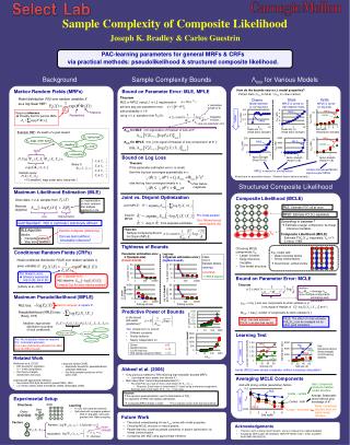
Sample Complexity of Composite Likelihood Joseph K. Bradley & Carlos Guestrin better better better PAC-learning parameters for general MRFs & CRFs via practical methods: pseudolikelihood & structured composite likelihood. ρmin = minj [ sum over components Ai which estimate θj of [ min eigval of Hessian of at θ* ]. MLE objective: MPLE-disjoint Mmax = maxj [ number of components Ai which estimate θj ]. MPLE MLE Sample Complexity Bounds Background Λmin for Various Models How do the bounds vary w.r.t. model properties? Markov Random Fields (MRFs) Bound on Parameter Error: MLE, MPLE Plotted: Ratio (Λmin for MLE) / (Λmin for other method) Model distribution P(X) over random variables X Chains Stars Grids as a log-linear MRF: Model diameter is not important. MPLE is worse for high-degree nodes. MPLE is worse for big grids. # parameters (length of θ) Features Requires inference. Provably hard for general MRFs. Parameters Probability of failure Avg. per-parameter error Λmin for MLE: min eigenvalue of Hessian of loss at θ*: Example MRF: the health of a grad student X4: losing hair? X2: bags under eyes? Λmin for MPLE: mini [ min eigval of Hessian of loss component i at θ* ]: X1: deadline? X3: sick? factor X5: overeating? Bound on Log Loss Combs (Structured MCLE) improve upon MPLE. MPLE is worse for strong factors. All plots are for associative factors. (Random factors behave similarly.) Max feature magnitude Structured Composite Likelihood Maximum Likelihood Estimation (MLE) Joint vs. Disjoint Optimization Composite Likelihood (MCLE) Given data: n i.i.d. samples from L2 regularization is more common. Our analysis applies to L1 & L2. Joint MPLE: Minimize objective: MLE: Estimate P(Y) all at once Yi MPLE: Estimate P(Yi|Y-i) separately Disjoint MPLE: Pro: Data parallel Con: Worse bound (extra factors |X|) Loss Regularization Something in between? Estimate a larger component, but keep inference tractable. Composite Likelihood (MCLE): Estimate P(YAi|Y-Ai) separately, YAi in Y. (Lindsay, 1988) Gold Standard: MLE is (optimally) statistically efficient. Theorem Sample Complexity Bound for Disjoint MPLE: • MLE Algorithm • Iterate: • Compute gradient. • Step along gradient. Hard to compute (inference). Can we learn without intractable inference? Binary X: YAi Theorem MLE or MPLE using L1 or L2 regularization achieve avg. per-parameter error with probability ≥ 1-δ using n i.i.d. samples from Pθ*(X): Example query: Tightness of Bounds = P( deadline | bags under eyes, losing hair ) • Choosing MCLE components YAi: • Larger is better. • Keep inference tractable. • Use model structure. Conditional Random Fields (CRFs) • E.g., model with: • Weak horizontal factors • Strong vertical factors • Good choice: vertical combs Parameter estimation error ≤ f(sample size) (looser bound) Log loss ≤ f(param estimation error) (tighter bound) Model conditional distribution P(X|E) over random variables X, given variables E: Log (base e) loss L1 param error Bound on Parameter Error: MCLE Chain. |X|=4. Random factors. Theorem (Lafferty et al., 2001) MLE Intuition: ρmin/Mmax = Average Λmin (over multiple components estimating each parameter) L1 param error bound Log loss bound, given params Combs - vertical Maximum Pseudolikelihood (MPLE) Pro: Model X, not E. Inference exponential only in |X|, not in |E|. Con: Z depends on E! Combs - both Training set size Training set size MPLE MLE loss: Hard to computereplace it! Compute Z(e) for every training example! Combs - horizontal Predictive Power of Bounds Pseudolikelihood (MPLE) loss: if (Besag, 1975) Is the bound still useful (predictive)? MCLE: The effect of a bad estimator P(XAi|X-Ai) can be averaged out by other good estimators. MPLE: One bad estimator P(Xi|X-i) can give bad results. Intuition: Approximate distribution as product of local conditionals. Theorem If the parameter estimation error ε is small, then the log loss converges quadratically in ε: else the log loss converges linearly in ε: • Yes! Actual error vs. bound: • Different constants • Similar behavior • Nearly independent of r X4: losing hair? X2: bags under eyes? X1: deadline? Learning Test X3: sick? Pro: No intractable inference required Pro: Consistent estimator Con: Less statistically efficient than MLE Con: No PAC bounds Λmin ratio Λmin ratio X5: overeating? MPLE MLE Grid. Associative factors (fixed strength). 10,000 training samples. combs Factor strength (Fixed |Y|=8) Model size |Y| (Fixed factor strength) Training time (sec) MPLE Log loss ratio (other/MLE) Related Work combs Random: X1 factor strength MPLE MPLE MPLE MPLE • Ravikumar et al. (2010) • PAC bounds for regression Yi ~ X with Ising factors. • Our theory is largely derived from this work. • Liang and Jordan (2008) • Asymptotic bounds for pseudolikelihood, composite likelihood. • Our finite sample bounds are of the same order. Grid size |X| Grid size |X| Abbeel et al. (2006) X2 Associative: Combs (MCLE) lower sample complexity--without increasing computation! otherwise • Only previous method for PAC-learning high-treewidth discrete MRFs. • (Low-degree factor graphs over discrete X.) • Main idea (their “canonical parameterization”): • Re-write P(X) as a ratio of many small factors P( XCi | X-Ci ). • Fine print: Each factor is instantiated 2|Ci| times using a reference assignment. • Estimate each small factor P( XCi | X-Ci ) from data. r=5 Chains. Random factors. 10,000 train exs. MLE (similar results for MPLE) Averaging MCLE Components • Learning with approximate inference • No previous PAC-style bounds for general MRFs, CRFs. • c.f.: Hinton (2002), Koller & Friedman (2009), Wainwright (2006) r=11 Best: Component structure matches model structure. Grid with strong vertical (associative) factors. r=23 Λmin ratio L1 param error Λmin ratio Theorem If the canonical parameterization uses the factorization of P(X), it is equivalent to MPLE with disjoint optimization. Average: Reasonable choice without prior knowledge of θ*. Experimental Setup Λmin Factor strength (Fixed |Y|=8) Model size |Y| (Fixed factor strength) Avg of from separate estimates Computing MPLE directly is faster. Our analysis covers their learning method. MPLE Grids Structures MPLE Learning Worst: Component structure does not match model structure. combs • 10 runs with separate datasets • Optimized with conjugate gradient • MLE on big grids: stochastic gradient with Gibbs sampling Stars combs L1 param error bound Chains Grid width Future Work Λmin ratio Λmin ratio Factors • Theoretical understanding of how Λmin varies with model properties. • Choosing MCLE structure on natural graphs. • Parallel learning: Lowering sample complexity of disjoint optimization via limited communication. • Comparing with MLE using approximate inference. 1/Λmin Acknowledgements • Thanks to John Lafferty, Geoff Gordon, and our reviewers for helpful feedback. • Funded by NSF Career IIS-0644225, ONR YIP N00014-08-1- 0752, and ARO MURI W911NF0810242. Factor strength (Fixed |Y|=8) Grid width (Fixed factor strength)