Maximum Likelihood
Maximum Likelihood. Likelihood The likelihood is the probability of the data given the model. Likelihood. If we flip a coin and get a head and we think the coin is unbiased, then the probability of observing this head is 0.5.

Maximum Likelihood
E N D
Presentation Transcript
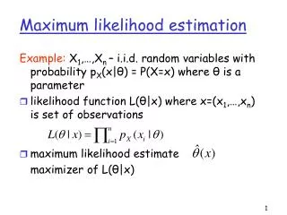
Likelihood The likelihood is the probability of the data given the model.
Likelihood If we flip a coin and get a head and we think the coin is unbiased, then the probability of observing this head is 0.5. If we think the coin is biased so that we expect to get a head 80% of the time, then the likelihood of observing this datum (a head) is 0.8. The likelihood of making some observation is entirely dependent on the model that underlies our assumption. The datum has not changed, our model has. Therefore under the new model the likelihood of observing the datum has changed.
Maximum Likelihood (ML) ML assumes a explicit model of sequence evolution. This is justifiable, since molecular sequence data can be shown to have arisen according to a stochastic process. ML attempts to answer the question: What is the probability that I would observe these data (amultiple sequence alignment) given a particular model of evolution (a tree and a process)?
Likelihood calculations In molecular phylogenetics, the data are an alignment of sequences We optimize parameters and branch lengths to get the maximum likelihood Each site has a likelihood The total likelihood is the product of the site likelihoods The maximum likelihood tree is the tree topology that gives the highest (optimized) likelihood under the given model. We use reversible models, so the position of the root does not matter.
What is the probability of observing a G nucleotide? • If we have a DNA sequence of 1 nucleotide in length and the identity of this nucleotide is G, what is the likelihood that we would observe this G? • In the same way as the coin-flipping observation, the likelihood of observing this G is dependent on the model of sequence evolution that is thought to underlie the data. • Model 1: frequency of G = 0.4 => likelihood(G) = 0.4 • Model 2: frequency of G = 0.1 => likelihood(G) = 0.1 • Model 3: frequency of G = 0.25 => likelihood(G) = 0.25
What about longer sequences? If we consider a gene of length 2 gene 1 GA The the probability of observing this gene is the product of the probabilities of observing each character Model frequency of G = 0.4 frequencyof A= 0.15 p(G) = 0.4 p(A)=0.15 Likelihood (GA) = 0.4 x 0.15 = 0.06
…or even longer sequences? gene 1 GACTAGCTAGACAGATACGAATTAC Model simple base frequency model p(A)=0.15; p(C)=0.2; p(G)=0.4; p(T)=0.25; (the sum of all probabilities must equal 1) Likelihood (gene 1) = 0.000000000000000018452813
Note about models You might notice that our model of base frequency is not the optimal model for our observed data. If we had used the following model p(A)=0.4; p(C) =0.2; p(G)= 0.2; p(T) = 0.2; The likelihood of observing the gene is L (gene 1) = 0.000000000000335544320000 L (gene 1) = 0.000000000000000018452813 The datum has not changed, our model has. Therefore under the new model the likelihood of observing the datum has changed.
Increase in model sophistication It is no longer possible to simply invoke a model that encompasses base composition, we must also include the mechanism of sequence change and stasis. There are two parts to this model - the tree and the process (the latter is confusingly referred to as the model, although both parts really compose the model).
Different Branch Lengths For very short branch lengths, the probability of a character staying the same is high and the probability of it changing is low. For longer branch lengths, the probability of character change becomes higher and the probability of staying the same is lower. The previous calculations are based on the assumption that the branch length describes one Certain Evolutionary Distance or CED. If we want to consider a branch length that is twice as long (2 CED), then we can multiply the substitution matrix by itself (matrix2).
Maximum Likelihood Two trees each consisting of single branch v = 0.1 I (A) II (C) v = 1.0 I (A) II (C) • v = mt m= mutation rate t = time
Jukes-Cantor model v = 0.1 I (A) II (C) v = 1.0 I (A) II (C)
I AACC II CACT
1 3 2 C 3 A 4 G 1 C 2 4 5 6 C C C C C C A A A G G G + p + … + p A T A C A T 1 j N 1 C G G A C A C G T T T A C 2 C A G A C A C C T C T A C 3 C G G A T A A G T T A A C 4 C G G A T A G C C T A G C L(j) = p
L(j) = p C C C C C C A A A G G G + p + … + p A A T T A C
Strengths of ML • Does not try to make an observation of sequence change and then a correction for superimposed substitutions. There is no need to ‘correct’ for anything, the models take care of superimposed substitutions. • Accurate branch lengths. • Each site has a likelihood. • If the model is correct, we should retrieve the correct tree (If we have long-enough sequences and a sophisticated-enough model). • You can use a model that fits the data. • ML uses all the data (no selection of sites based on informativeness, all sites are informative). • ML can not only tell you about the phylogeny of the sequences, but also the process of evolution that led to the observations of today’s sequences.
Weaknesses of ML • Can be inconsistent if we use models that are not accurate. • Model might not be sophisticated enough • Very computationally-intensive. Might not be possible to examine all models (substitution matrices, tree topologies).
Models • You can use models that: Deal with different transition/transversion ratios. Deal with unequal base composition. Deal with heterogeneity of rates across sites. Deal with heterogeneity of the substitution process (different rates across lineages, different rates at different parts of the tree). • The more free parameters, the better your model fits your data (good). • The more free parameters, the higher the variance of the estimate (bad).
Choosing a Model Don’t assume a model, rather find a model that fits your data. Models often have “free” parameters. These can be fixed to a reasonable value, or estimated by ML. The more free parameters, the better the fit (higher the likelihood) of the model to the data. (Good!) The more free parameters, the higher the variance, and the less power to discriminate among competing hypotheses. (Bad!) We do not want to over-fit the model to the data
What is the best way to fit a line (a model) through these points? • How to tell if adding (or removing) a certain parameter is a good idea? • Use statistics • The null hypothesis is that the presence or absence of the parameter makes no difference • In order to assess signifcance you need a null distribution
We have some DNA data, and a tree. Evaluate the data with 3 different models. model ln likelihood ∆ JC -2348.68 K2P -2256.73 91.95 GTR -2254.94 1.79 Evaluations with more complex models have higher likelihoods The K2P model has 1 more parameter than the JC model The GTR model has 4 more parameters than the K2P model Are the extra parameters worth adding?
You can use the 2 approximation to assess significance of adding parameters K2P vs GTR JC vs K2P We have generated many true null hypothesis data sets and evaluated them under the JC model and the K2P model. 95% of the differences are under 2.The statistic for our original data set was 91.95, and so it is highly significant. In this case it is worthwhile to add the extra parameter (tRatio). We have generated many true null hypothesis data sets and evaluated them under the K2P model and the GTR model. The statistic for our original data set was 1.79, and so it is not signifcant. In this case it is not worthwhile to add the extra parameters.
Maximum likelihood Search for tree that maximizes the chance of seeing the data (P (Data | Tree)) Bayesian Inference Search for tree that maximizes the chance of seeing the tree given the data (P (Tree | Data))
Bayesian Phylogenetics Maximize the posterior probability of a tree given the aligned DNA sequences Two steps - Definition of the posterior probabilities of trees (Bayes’ Rule) - Approximation of the posterior probabilities of trees Markov chain Monte Carlo (MCMC) methods
Bayesian Inference 90 10
Markov Chain Monte Carlo Methods Posterior probabilities of trees are complex joint probabilities that cannot be calculated analytically. Instead, the posterior probabilities of trees are approximated with Markov Chain Monte Carlo(MCMC) methods that sample trees from their posterior probability distribution.
MCMC A way of sampling / touring a set of solutions,biased by their likelihood 1 Make a random solution N1 the current solution 2 Pick another solution N2 3 If Likelihood (N1 < N2) then replace N1 with N2 4 Else if Random (Likelihood (N2) / Likelihood (N1)) then replace N1 with N2 5 Sample (record) the current solution 6 Repeat from step 2


