Maximum likelihood
Maximum likelihood. The maximum likelihood criterion. The optimal tree is that which would be most likely to give rise to the observed data (under a given model of evolution). An outline of the ML approach: Consider one character, i. (It is useful to arbitrarily root the tree).

Maximum likelihood
E N D
Presentation Transcript
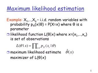
The maximum likelihood criterion • The optimal tree is that which would be most likely to give rise to the observed data (under a given model of evolution)
An outline of the ML approach:Consider one character, i (It is useful to arbitrarily root the tree)
Sum across all possible histories for i There are 4(n-2) arrangements for n taxa
We calculate the likelihood of getting the observed states = L(i) G G A G t2 t3 t4 t5 A t1 A L(i) = PA x PA-A(t1)x PA-G(t2)x PA-G(t3)x PA-A(t4)x PA-G(t5)
Multiply across all sites (assume independence) L will be very small(lnL will be a large negative number)
Tree searching • Search for the set of branch-lengths that maximize L (= lower -lnL score) • Record that score • Search for tree topologies with the best score Time consuming!
Issues glossed over • Where do we get Pn - the probability of state n at the arbitrary root node? • Equiprobable (25%) • Empirical (frequency in the entire matrix) • Estimated (optimized by ML on each tree) • Where do we get Pi-j(t) - the probability of going from state i to state j in time t?
Typical Simplifying Assumptions • Stationarity • Reversibility • Site independence • Markovian process (no “memory”)
The simplest model of molecular evolution: Jukes-Cantor Instantaneous rate matrix (Q-matrix)
Calculating probabilities of change • To convert the Q matrix into a matrix giving the probability of starting at state i and ending in state j, t time units later uses the formula: P(t)= eQt
The simplest model of molecular evolution: Jukes-Cantor Substitution probability matrix (P-matrix)
Worked example A G 0.02 0.01 0.03 0.01 0.02 A G
Worked example A G 0.02 0.01 A A 0.03 0.01 0.02 A G
Worked example A G Non-change = ¼ +¾e-t Change = ¼ - ¼e-t 0.02 0.01 A A 0.03 0.01 0.02 A G
Worked example A G Non-change = ¼ +¾e-t Change = ¼ - ¼e-t 0.02 0.01 A A 0.03 0.01 0.02 A G L =0.25(¼ +¾e-0.02) (¼ +¾e-0.02) (¼ +¾e-0.03) (¼ - ¼e-0.01) (¼ - ¼e-0.01)
Worked example A G Non-change = ¼ +¾e-t Change = ¼ - ¼e-t 0.02 0.01 A A 0.03 0.01 0.02 A G L =(¼ +¾e-0.02) (¼ +¾e-0.02) (¼ +¾e-0.03) (¼ - ¼e-0.01) (¼ - ¼e-0.01) L =(0.985149) (0.985149) (0.977834) (0.0024875) (0.0024875)
Worked example A G Non-change = ¼ +¾e-t Change = ¼ - ¼e-t 0.02 0.01 A A 0.03 0.01 0.02 A G L =(¼ +¾e-0.02) (¼ +¾e-0.02) (¼ +¾e-0.03) (¼ - ¼e-0.01) (¼ - ¼e-0.01) L =(0.985149) (0.985149) (0.977834) (0.0024875) (0.0024875) L = 0.00000587232 or 5.87232 x 10⁻⁶
Worked example A G Non-change = ¼ +¾e-t Change = ¼ - ¼e-t 0.02 0.01 A G 0.03 0.01 0.02 A G L =(¼ +¾e-0.02) (¼ +¾e-0.02) (¼ - ¼e-0.03) (¼ +¾e-0.01) ¼ +¾e-0.01) L =(0.985149) (0.985149) (0.0073886) (0.9925373) (0.9925373) L = 0.007064163 or 7.064163 x 10⁻³
Sum over all other combinations • AA = 5.87232x10⁻⁶ • AG = 7.064163x10⁻³ • AC = • AT = • GA = • GG = • GC = • GT = • CA = • CG = • CC = • CT = • TA = • TG = • TC = • TT =
Sum over all other combinations • AA = NC-NC-C • AG = NC-C-NC • AC = NC-C-C • AT = NC-C-C • GA = C-C-C • GG = C-NC-NC • GC = C-C-C • GT = C-C-C • CA = C-C-C • CG = C-C-NC • CC = C-NC-C • CT = C-C-C • TA = C-C-C • TG = C-C-NC • TC = C-C-C • TT = C-NC-C
Sum over all other combinations • AA = 5.87232x10⁻⁶ • AG = 7.064163x10⁻³ • AC = 4.43719x10⁻⁸ • AT = 4.43719x10⁻⁸ • GA = 1.1204x10⁻¹² • GG = 2.36063x10⁻⁵ • GC = 1.1204x10⁻¹² • GT = 1.1204x10⁻¹² • CA = 1.1204x10⁻¹² • CG = 1.78372x10⁻⁷ • CC = 1.48277x10⁻¹² • CT = 1.1204x10⁻¹² • TA = 1.1204x10⁻¹² • TG = 1.78372x10⁻⁷ • TC = 1.1204x10⁻¹² • TT = 1.48277x10⁻¹⁰
Sum over all other combinations = 7.09 x 10⁻³ • AA = 5.87232x10⁻⁶ • AG = 7.064163x10⁻³ • AC = 4.43719x10⁻⁸ • AT = 4.43719x10⁻⁸ • GA = 1.1204x10⁻¹² • GG = 2.36063x10⁻⁵ • GC = 1.1204x10⁻¹² • GT = 1.1204x10⁻¹² • CA = 1.1204x10⁻¹² • CG = 1.78372x10⁻⁷ • CC = 1.48277x10⁻¹² • CT = 1.1204x10⁻¹² • TA = 1.1204x10⁻¹² • TG = 1.78372x10⁻⁷ • TC = 1.1204x10⁻¹² • TT = 1.48277x10⁻¹⁰
Likelihood scores • Raw likelihood of the data at this site given this tree and branch lengths and model = 0.25(7.09 x 10⁻³) • Log-likelihood = -6.334787983
What does this number mean? • -6.334787983 = The log-likelihood of the data (tip values) given: • This tree topology • These branch lengths • The model of molecular evolution
Multiplying across sites To make it easier, we can lump characters with the same “pattern” lnL = [lnL (0000)]N(0000) + [lnL (0001)]N(0001) + [lnL (0010)]N(0010) + [lnL (0100)]N(0100) + [lnL (0111)]N(0111) + [lnL (0011)]N(0011) + [lnL (0101]N(0101)) + [lnL (0110)]N(0110)
What branch lengths should we assume? • Under the principle of maximum likelihood, we use the set of branch lengths that maximize the likelihood • Once we find those branch lengths, the likelihood score is taken as being the likelihood of the data given this tree topology


