Notes 6: Constraint Satisfaction Problems
Notes 6: Constraint Satisfaction Problems. ICS 270A Spring 2003. Summary. The constraint network model Variables, domains, constraints, constraint graph, solutions Examples: graph-coloring, 8-queen, cryptarithmetic, crossword puzzles, vision problems,scheduling, design

Notes 6: Constraint Satisfaction Problems
E N D
Presentation Transcript
Notes 6: Constraint Satisfaction Problems ICS 270A Spring 2003
Summary • The constraint network model • Variables, domains, constraints, constraint graph, solutions • Examples: • graph-coloring, 8-queen, cryptarithmetic, crossword puzzles, vision problems,scheduling, design • The search space and naive backtracking, • Line drawing interpretation • Class scheduling • The constraint graph • Approximation consistency enforcing algorithms • arc-consistency, • AC-1,AC-3 • Backtracking strategies • Forward-checking, dynamic variable orderings • Special case: solving tree problems
E A B red green red yellow green red green yellow yellow green yellow red A D B F G C Constraint Satisfaction Example: map coloring Variables - countries (A,B,C,etc.) Values - colors (e.g., red, green, yellow) Constraints:
Examples • Cryptarithmetic • SEND + • MORE = MONEY • n - Queen • Crossword puzzles • Graph coloring problems • Vision problems • Scheduling • Design
A network of binary constraints • Variables • Domains • of discrete values: • Binary constraints: • which represent the list of allowed pairs of values, Rij is a subset of the Cartesian product: . • Constraint graph: • A node for each variable and an arc for each constraint • Solution: • An assignment of a value from its domain to each variable such that no constraint is violated. • A network of constraints represents the relation of all solutions.
4 2 Example 1: The 4-queen problem • Standard CSP formulation of the problem: • Variables: each row is a variable. Place 4 Queens on a chess board of 4x4 such that no two queens reside in the same row, column or diagonal. 1 2 3 4 Q Q Q Q Q Q Q Q Q Q Q Q • Domains: ( ) • Constraints: There are = 6 constraints involved: • Constraint Graph :
The search space • Definition: given an ordering of the variables • a state: • is an assignment to a subset of variables that is consistent. • Operators: • add an assignment to the next variable that does not violate any constraint. • Goal state: • a consistent assignment to all the variables.
Backtracking • Complexity of extending a partial solution: • Complexity of consistent O(e log t), t bounds tuples, e constraints • Complexity of selectvalue O(e k log t)
Approximation algorithms • Arc-consistency (Waltz, 1972) • Path-consistency (Montanari 1974, Mackworth 1977) • I-consistency (Freuder 1982) • Transform the network into smaller and smaller networks.
Arc-consistency X Y 1, 2, 3 1, 2, 3 1 X, Y, Z, T 3 X Y Y = Z T Z X T = 1, 2, 3 1, 2, 3 T Z
1 3 2 3 Arc-consistency X Y 1 X, Y, Z, T 3 X Y Y = Z T Z X T = T Z • Incorporated into backtracking search • Constraint programming languages powerful approach for modeling and solving combinatorial optimization problems.
Arc-consistency algorithm domain of x domain of y Arc is arc-consistent if for any value of there exist a matching value of Algorithm Revise makes an arc consistent Begin 1. For each a in Di if there is no value b in Di that matches a then delete a from the Dj. End. Revise is , k is the number of value in each domain.
Algorithms for arc-consistency • A network is arc-consistent if all its arcs are arc-consistent AC-1 begin 1. until there is no change do 2. For every directed arc (X,Y) Revise(X,Y) end Complexity: , e is the number of arcs, n number of variables, k is the domain size. Mackworth and Freuder, 1986 showed an algorithm Mohr and Henderson, 1986:
Algorithm AC-3 • Complexity • Begin • 1. Q <--- put all arcs in the queue in both directions • 2. While Q is not empty do, • 3. Select and delete an arc from the queue Q • 4. Revise • 5. If Revise cause a change then add to the queue all arcs that touch Xi (namely (Xi,Xm) and (Xl,Xi)). • 6. end-while • end • Processing an arc requires O(k^2) steps • The number of times each arc can be processed is 2·k • Total complexity is
Improving backtracking • Before search: (reducing the search space) • Arc-consistency, path-consistency • Variable ordering (fixed) • During search: • Look-ahead schemes: • value ordering, • variable ordering (if not fixed) • Look-back schemes: • Backjump • Constraint recording • Dependency-directed backtacking
Look-ahead: value orderings • Intuition: • Choose value least likely to yield a dead-end • Approach: apply propagation at each node in the search tree • Forward-checking • (check each unassigned variable separately • Maintaining arc-consistency (MAC) • (apply full arc-consistency) • Full look-ahead • One pass of arc-consistency (AC-1) • Partial look-ahead • directional-arc-consistency
Backtracking • Complexity of extending a partial solution: • Complexity of consistent O(e log t), t bounds tuples, e constraints • Complexity of selectvalue O(e k log t)
Forward-checking • Complexity of selectValue-forward-checking at each node:
Dynamic value ordering (LVO) Use constraint propagation to rank order the promise in non-rejected values. Example: look-ahead value ordering (LVO) is based of forward-checking propagation LVO uses a heuristic measure to transform this information to ranking of the values Empirical work shows the approach is cost-effective only for large and hard problems.
Look-ahead: variable ordering • Dynamic search rearangement (Bitner and Reingold, 1975)(Purdon,1983): • Choose the most constrained variable • Intuition: early discovery of dead-ends
Implementing look-aheads • Cost of node generation should be reduced • Solution: keep a table of viable domains for each variable and each level in the tree. • Space complexity • Node generation = table updating
Look-back: backjumping • Backjumping: Go back to the most recently culprit. • Learning: constraint-recording, no-good recording.
The cycle-cutset method • An instantiation can be viewed as blocking cycles in the graph • Given an instantiation to a set of variables that cut all cycles (a cycle-cutset) the rest of the problem can be solved in linear time by a tree algorithm. • Complexity (n number of variables, k the domain size and C the cycle-cutset size):
Propositional Satisfiability Example: party problem • If Alex goes, then Becky goes: • If Chris goes, then Alex goes: • Query: Is it possible that Chris goes to the party but Becky does not?
Look-ahead for SAT(Davis-Putnam, Logeman and Laveland, 1962)
Approximating Conditioning: Local Search • Problem: complete (systematic, exhaustive) search can be intractable (O(exp(n)) worst-case) • Approximation idea: explore only parts of search space • Advantages: anytime answer; may “run into” a solution quicker than systematic approaches • Disadvantages: may not find an exact solution even if there is one; cannot detect that a problem is unsatisfiable
Simple “greedy” search 1. Generate a random assignment to all variables 2. Repeat until no improvement made or solution found: // hill-climbing step 3. flip a variable (change its value) that increases the number of satisfied constraints Easily gets stuck at local maxima
GSAT – local search for SAT(Selman, Levesque and Mitchell, 1992) • For i=1 to MaxTries • Select a random assignment A • For j=1 to MaxFlips • if A satisfies all constraint, return A • else flip a variable to maximize the score • (number of satisfied constraints; if no variable • assignment increases the score, flip at random) • end • end Greatly improves hill-climbing by adding restarts and sideway moves
WalkSAT (Selman, Kautz and Cohen, 1994) Adds random walk to GSAT: With probability p random walk – flip a variable in some unsatisfied constraint With probability 1-p perform a hill-climbing step Randomized hill-climbing often solves large and hard satisfiable problems
Other approaches • Different flavors of GSAT with randomization (GenSAT by Gent and Walsh, 1993; Novelty by McAllester, Kautz and Selman, 1997) • Simulated annealing • Tabu search • Genetic algorithms • Hybrid approximations: elimination+conditioning