Operational configuration Main features of the operational ALADIN/HU model

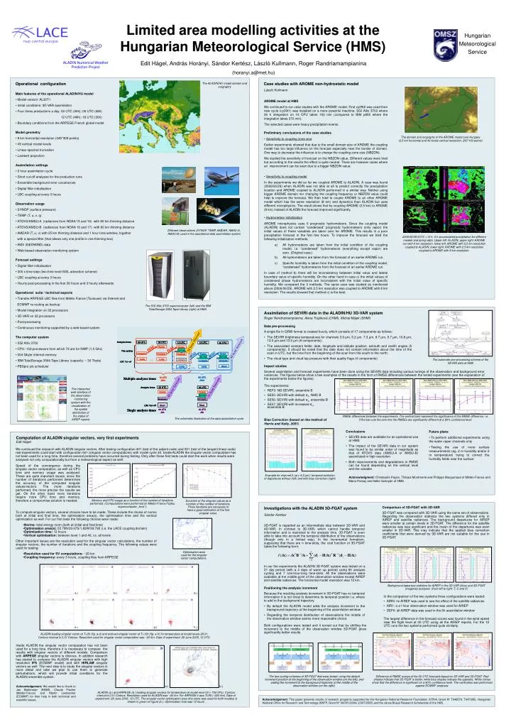
1. 14 14 23 23 65 65 41 41 20 20 13 13 15 15 14 14 23 23 65 65 41 41 20 20 13 13 15 15 54 hour forecast 54 hour forecast 54 hour forecast 54 hour forecast Analysis times Analysis times Analysis times Analysis times 00 UTC 00 UTC 00 UTC 00 UTC 06 UTC 06 UTC 06 UTC 06 UTC 12 UTC 12 UTC 12 UTC 12 UTC 18 UTC 18 UTC 18 UTC 18 UTC 00 UTC 00 UTC 00 UTC 00 UTC Guess Guess Guess Guess Guess Guess Guess Guess fcst fcst fcst fcst fcst 48 hour forecast 48 hour forecast 48 hour forecast 48 hour forecast fcst fcst fcst fcst fcst 6 h 6 h 6 h 6 h 6 h 6 h 6 h 6 h 6 h 6 h 3d 3d 3d 3d - - - - Var Var Var Var The cycling The cycling The cycling The cycling Analysis Analysis Analysis Analysis Guess Guess Guess Guess Analysis Analysis Analysis Analysis Guess Guess Guess Guess Analysis Analysis Analysis Analysis fcst fcst fcst fcst fcst fcst fcst fcst fcst 6h 6h 6h 6h 6h 6h 6h 6h 6h 3d 3d 3d 3d - - - - Var Var Var Var 3d 3d 3d 3d - - - - Var Var Var Var … … … … Long Long Long Long Long Long Long Long Short Short Short Short Analysis Analysis Analysis Analysis Analysis Analysis Analysis Analysis LBC Cut LBC Cut LBC Cut LBC Cut - - - - off off off off … … … … Short Short Short Short Long Long Long Long Long Long Long Long 00 UTC 00 UTC 00 UTC 00 UTC 12 UTC 12 UTC 12 UTC 12 UTC Multiple analyses times Multiple analyses times Multiple analyses times Multiple analyses times Jobs Jobs Jobs Jobs Jobs Jobs Jobs Jobs 18 hour forecast 36 hour forecast 18 hour forecast 18 hour forecast 48 hour forecast 48 hour forecast 48 hour forecast 48 hour forecast 06 UTC 06 UTC 06 UTC 06 UTC Analysis times Analysis times Analysis times Analysis times 06 UTC 06 UTC 06 UTC 06 UTC Guess Guess Guess Guess Guess Guess Guess Guess 3d 3d 3d 3d - - - - Var Var Var Var Analysis Analysis Analysis Analysis Analysis Analysis Analysis Analysis Short Short Short Short LBC Cut LBC Cut LBC Cut LBC Cut - - - - off off off off Short Short Short Short Single analysis times Single analysis times Single analysis times Single analysis times 06 UTC 06 UTC 06 UTC 06 UTC 18 UTC 18 UTC 18 UTC 18 UTC Job Job Job Job Job Job Job Job b.) d.) a.) c.) f.) h.) e.) g.) Limited area modelling activities at the Hungarian Meteorological Service (HMS) Hungarian Meteorological Service ALADIN Numerical Weather Prediction Project Edit Hágel, András Horányi, Sándor Kertész, László Kullmann, Roger Randriamampianina (horanyi.a@met.hu) Case studies with AROME non-hydrostatic model László Kullmann • Operational configuration • Main features of the operational ALADIN/HU model • Model version: AL30T1 • Initial conditions: 3D-VAR assimilation • Four times productions a day: 00 UTC (54h); 06 UTC (48h) • 12 UTC (48h); 18 UTC (36h) • Boundary conditions from the ARPEGE French global model • Model geometry • 8 km horizontal resolution (349*309 points) • 49 vertical model levels • Linear spectral truncation • Lambert projection • Assimilation settings • 6 hour assimilation cycle • Short cut-off analyses for the production runs • Ensemble background error covariances • Digital filter initialisation • LBC coupling at every 3 hours • Observation usage • SYNOP (surface pressure) • TEMP (T, u, v, q) • ATOVS/AMSU-A (radiances from NOAA 15 and 16) with 80 km thinning distance • ATOVS/AMSU-B (radiances from NOAA 16 and 17) with 80 km thinning distance • AMDAR (T, u, v) with 25 km thinning distance and 1 hour time-window, together • with a special filter (that allows only one profile in one thinning-box) • AMV (GEOWIND) data • Web-based observation monitoring system • Forecast settings • Digital filter initialisation • 300 s time-step (two-time level SISL advection scheme) • LBC coupling at every 3 hours • Hourly post-processing in the first 36 hours and 3 hourly afterwards • Operational suite / technical aspects • Transfer ARPEGE LBC files from Météo France (Toulouse) via Internet and • ECMWF re-routing as backup • Model integration on 32 processors • 3D-VAR on 32 processors • Post-processing • Continuous monitoring supported by a web based system • The computer system • SGI Altix 3700 • CPU: 152 processors from which 72 are for NWP (1,5 Ghz) • 304 Gbyte internal memory • IBM TotalStorage 3584 Tape Library (capacity: ~ 30 Tbyte) • PBSpro job scheduler The ALADIN/HU model domain and orography AROME model at HMS We continued to run case studies with the AROME model. First cy29t2 was used then new cycle (cy30t1) was installed on a more powerful machine: SGI Altix 3700 where 24h integration on 16CPU takes 150min (compared to IBM p655 where the integration takes 270min). The selected cases were heavy precipitation events. Preliminary conclusions of the case studies • Sensitivity to coupling zone size • Earlier experiments showed that due to the small domain size of AROME the coupling model has too large influence on the forecast especially near the border of domain. One way to decrease the influence is to change the coupling zone size (NBZON). • We studied the sensitivity of forecast on the NBZON value. Different values were tried but according to the results the effect is quite neutral. There are however cases where an improvement can be seen due to a bigger NBZON value. The domain and orography of the AROME model over Hungary (2,5 km horizontal and 49 levels vertical resolution, 250*160 points) • Sensitivity to coupling model • In the experiments we did so far we coupled AROME to ALADIN. A case was found (2006/06/29) when ALADIN was not able at all to predict correctly the precipitation location and AROME coupled to ALADIN performed in a similar way. Neither using bigger AROME domain nor changing the coupling frequency or NBZON value could help to improve the forecast. We then tried to couple AROME to an other AROME model which has the same resolution (8km) and dynamics than ALADIN but uses different microphysics. The result shows that by coupling AROME(2.5km) to AROME(8km) instead of ALADIN the forecast improved significantly. • Hydrometeor initialization • AROME microphysics uses 6 prognostic hydrometeors. Since the coupling model (ALADIN) does not contain “condensed” prognostic hydrometeors (only vapor) the initial values of these variables are taken zero for AROME. This results in a poor precipitation forecast in the first few hours. To improve the forecast we tried the following initialization methods: • All hydrometeors are taken from the initial condition of the coupling model, i.e. “condensed” hydrometeors (everything except vapor) are zero. (Original case.) • All hydrometeors are taken from the forecast of an earlier AROME run. • Specific humidity is taken from the initial condition of the coupling model, “condensed” hydrometeors from the forecast of an earlier AROME run. • In case of method b) there will be inconsistency between initial value and lateral boundary value of specific humidity. On the other hand in case c) the initial values of condensed phase hydrometeors are inconsistent with the initial value of specific humidity. We compared the 3 methods. The same case was studied as mentioned above (2006/06/29). AROME with 2.5km resolution was coupled to AROME with 8km resolution. The results showed that method c) is the best. Different observations (SYNOP, TEMP, AMDAR, AMSU-A, AMSU-B) used in the operational data assimilation system 2006/06/29 0UTC +12h, 6h accumulated precipitation for different models and synop data. Upper left: ALADIN, upper right: AROME run with 8km resolution, lower left: AROME with 2.5km resolution coupled to ALADIN, lower right: AROME with 2.5km resolution coupled to AROME with 8km resolution. The SGI Altix 3700 supercomputer (left) and the IBM TotalStorage 3584 Tape Library (right) at HMS. Assimilation of SEVIRI data in the ALADIN/HU 3D-VAR system Roger Randriamampianina, Alena Trojáková (CHMI), Michal Májek (SHMI) • Data pre-processing • A single file in GRIB format is created hourly, which consists of 17 components as follows: • The SEVIRI brightness temperatures for channels 3.9 µm, 6.2 µm, 7.3 µm,8.7 µm, 9.7 µm, 10.8 µm, 12.0 µm and 13.4 µm (8 components); • The associated constant fields: date, longitude and latitude position, azimuth and zenithangles (5 components). It should be noted that the date does not contain information about the time of the scan in UTC, but the time from the beginning of the scan from thesouth to the north; • The cloud type and cloud top pressure with their quality flags (4 components) The automatic pre-processing scheme of the SEVIRI data at HMS Impact studies Several assimilation and forecast experiments have been done using the SEVIRI data including various tunings of the observation and background error variances. The figures below show a few examples of the results in the form of RMSE differences between the tested experiments (see the explanation of the experiments below the figures). • The experiments: • REF3: NO SEVIRI, ensemble B • SE55: SEVIRI with default σo, NMC B • SE56: SEVIRI with default σo, ensemble B • SE57: SEVIRI with increased σo, ensemble B The interactive web interface of the observation monitoring system with the visualization of the spatial distribution of the status of AIREP reports RMSE differences between the experiments. The vertical bars represent the significance of the RMSE difference, i.e. if the bar cuts the zero line the RMSEs are significantly different at a 90% confidence level. The schematic illustration of the data assimilation cycle Bias Correction (based on the method of Harris and Kelly, 2001) • Future plans • To perform additional experiments using the water vapor channels only • Testing the use of more surface measurements (eg. 2m humidity and/or 2 m temperature) trying to correct the humidity fields near the surface • Conclusions • SEVIRI data are available for an operational use at HMS • The impact of the SEVIRI data in our system was found to be similar order of magnitude as that of ATOVS data (AMSU-A or AMSU-B) assimilated in high resolution • Both improvements and degradations in RMSE can be found depending on the vertical level and the variable Computation of ALADIN singular vectors, very first experiments Edit Hágel We continued the research with ALADIN singular vectors. After testing configuration 401 (test of the adjoint code) and 501 (test of the tangent linear code) real experimentscould start with configuration 601 (singular vector computations) with model cycle 30. Inside ALADIN the singular vector computation has not been used for a long time, therefore several problems have occurred during testing. Only after these first tests could start the work when results were analysed not only computationally but from a meteorological aspect as well. Speed of the convergence during the singular vector computation, as well as CPU time and memory usage was analysed. These are quite important issues, since the number of iterations performed determines the accuracy of the computed singular values/vectors. The more iterations performed, the more precise the results we get. On the other hand more iterations require more CPU time and memory, therefore a compromise solution is needed. Example for channel 2 (w.v. 6.2 µm): temporal evolution of departures without (left) and with bias correction (right) Acknowledgment: Christophe Payan, Thibaut Montmerle and Philippe Marguinaud of Météo-France and Maria Putsay and Ildikó Szenyán of HMS Memory and CPU usage as a function of the number of iterations performed. (Computations were performed on Météo-France Fujitsu supercomputer, „tora”.) Evolution of the singular values as a function of the number of iterations. Three iterations are necessary to have a good estimation of the first singular value. Comparison of 3D-FGAT with 3D-VAR 3D-FGAT was compared with 3D-VAR using the same set of observations. Regarding the observation statistics the two systems differed only in AIREP and satellite radiances. The background departures for AIREP were smaller at certain levels in 3D-FGAT. The difference for the satellite radiances was less significant and the mean of the departures was even smaller in 3D-VAR. This may indicate that the applied bias correction coefficients that were derived by 3D-VAR are not suitable for the use in 3D-FGAT. Investigations with the ALADIN 3D-FGAT system • To compute singular vectors, several choices have to be made. These include the choice of norms both at initial and final time, the optimisation area(s), the optimisation time and the vertical optimization as well. For our first tests the following choices were made: • Norms: total energy norm (both at initial and final time) • Optimisation area(s): 55.78N/33.67S/1.83W/39.79E (i.e. the LACE coupling domain) • Optimisation time: 12 hours • Vertical optimisation: between level 1 and 46, i.e. all levels • Other important issues are the resolution used for the singular vector calculations, the number of singular vectors, the number of iterations and the coupling frequency. The following values were used for testing: • Resolution used for SV computations: ~20 km • Coupling frequency: every 3 hours, coupling files from ARPEGE Sándor Kertész 3D-FGAT is regarded as an intermediate step between 3D-VAR and 4D-VAR. In contrast to 3D-VAR, which cannot handle temporal information and is restricted to the analysis time, 3D-FGAT is even able to take into account the temporal distribution of the observations (though only in a limited way). In the incremental formalism, supposing that there are n time-slots, the cost function of 3D-FGAT takes the following form: Optimisation area used for the singular vector computations. In our the experiments the ALADIN 3D-FGAT system was tested on a 21 day period (with a 4 days of warm up period) using 6h analysis cycling and 7 one-hour-long time-slots. All the observations were available at the middle point of the observation window except AIREP and satellite radiances. The horizontal model resolution was 12 km. Background departure statistics for AIREP in the 3D-VAR (blue) and 3D-FGAT (magenta) analyses (from left to right: T, U and V) Positioning the analysis increment Because the resulting analysis increment in 3D-FGAT has no temporal information it is not trivial to determine its temporal position i.e. where to add to the background trajectory. • In the comparison of the two systems three configurations were tested: • AIRN: no AIREP was used to see the effect of the satellite radiances • AIR1: a ±1 hour observation window was used for AIREP • DEF6: all AIREP data was used in the 6h assimilation window • By default the ALADIN model adds the analysis increment to the background trajectory at the beginning of the assimilation window • Regarding the temporal distribution of observations the middle of the observation window seems more reasonable choice The largest difference in the forecast scores was found in the wind speed near the flight level at 00 UTC using all the AIREP reports. For the 12 UTC runs the two systems performed quite similarly. Both configurations were tested and it turned out that by shifting the increment to the middle of the observation window 3D-FGAT gives significantly better results. ALADIN leading singular vector at T+0h (fig. a-d) and evolved singular vector at T+12h(fig. e-h) for temperature at model levels28-31. Contour interval is 0.01 Celsius. Resolution used for singular vector computation was ~20 km. Date of experiment: 28 June 2006, 12 UTC. Inside ALADIN the singular vector computation has not been used for a long time, therefore it is necessary to compare the results with singular vectors of different models. Comparison with ARPEGE singular vectors is obvious. In addition research has started to compare the ALADIN singular vectors with high resolution IFS (ECMWF model) and with HIRLAM singular vectors as well. The next step is to study the singular vectors in more detail and later we plan to use them to generate perturbations, which will provide initial conditions for the ALADIN ensemble system. Difference of RMSE scores of the 00 UTC forecasts based on 3D-VAR and3D-FGAT. Red shades indicate that 3D-FGAT is better, while blue shades indicate the opposite. White circles show thatthe difference is significant on a 90% confidence level.The verification was performed against ECMWF analyses. The two cycling schemes of 3D-FGAT that were tested: using the default increment position at the beginning of the observation window (on the left), and adding the increment to the background trajectory at the middle of the observation window (on the right). a.) Acknowledgement: We would like to thank to Jan Barkmeijer (KNMI), Claude Fischer (Météo-France) and Martin Leutbecher (ECMWF) for their help in both technical and scientific issues. b.) ALADIN (a.) and ARPEGE (b.) leading singular vectors for temperature at model level 32 (~730 hPa). Contour interval is 0.01 Celsius. Resolution used for ALADIN was ~20 km. For ARPEGE it was TL95 (~220 km). Date of experiment: 28 June 2006, 12 UTC. The singular vector optimization area (the same was used for both models) is shown in green on figure (b.). Optimization time was 12 hours. Acknowledgement: This paper presents results of research programs supported by the Hungarian National Research Foundation (OTKA, Grant N° T049579, T047295), Hungarian National Office for Research and Technology(NKFP, Grant N° 3A/051/2004, 2/007/2005) and the János Bolyai Research Scholarship of the HAS.