Simulating Normal Random Variables
Simulating Normal Random Variables. Simulation can provide a great deal of information about the behavior of a random variable. Simulating Normal Random Variables. Two types of simulations (1) Generating fixed values - Uses Random Number Generation (2) Generating changeable values

Simulating Normal Random Variables
E N D
Presentation Transcript
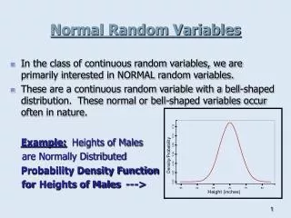
Simulating Normal Random Variables Simulation can provide a great deal of information about the behavior of a random variable
Simulating Normal Random Variables • Two types of simulations (1) Generating fixed values - Uses Random Number Generation (2) Generating changeable values - Uses NORMINV function
Simulating Normal Random Variables • Fixed Values • Random Number Generation is found under Tools/Data Analysis • Values will never change • Useful if you need to show how your specific results are tabulated
Simulating Normal Random Variables • Sample: Number of columns Number of rows Type of distribution Mean Standard Deviation (Leave blank) Cell where data is placed
Simulating Normal Random Variables • Ex. Generate a fixed sample of data containing 25 values that has a normal distribution with a mean of 13 and a standard deviation of 4.6
Simulating Normal Random Variables • Ex. Generate a fixed sample of data containing 30 values in cells A1:F5 that has a normal distribution with a mean of 81 and a standard deviation of 21
Simulating Normal Random Variables • Ex. Suppose X is a normal random variable whose mean is 140 and standard deviation 18. Find a 90% confidence interval for sample mean for samples of size 6 of the random variable X.
Simulating Normal Random Variables • Ex. Generate a fixed sample of data containing 1000 samples of size 6 each, where the values in the sample represent final exam scores and have a normal distribution with a mean of 140 and a standard deviation of 18.
Simulating Normal Random Variables • Ex. For the 1000 samples created in the previous example, find the sample mean for each. Then use the DCOUNT function to determine how many of the 1000 sample mean values lie within the 90% confidence interval. • Soln: Approximately 90% of the values should lie within the 90% confidence interval.
Simulating Normal Random Variables • Caution! Occasionally the values Random Number Generation gives might yield poor values • These values are more than 6 standard deviations from the mean • Find the max and min to be certain the values are within the appropriate range, replacing any values outside of the range
Simulating Normal Random Variables • Changeable Values • NORMINV function • Values will change by pressing F9 or by setting calculation in automatic mode • Useful if you want several samples to average (eliminates a small number of poor values)
Simulating Normal Random Variables • NORMINV will be used to run simulations for the project • Sample data looks similar to Random Number Generation sample data • Difference is that values can change by pressing F9
Simulating Normal Random Variables • Sample: - Any number between 0 and 1 (Use RAND( ) for random values) - Mean - Standard Deviation
Simulating Normal Random Variables • Ex. Generate a changeable sample of data containing 30 values in cells A1:F5 that has a normal distribution with a mean of 81 and a standard deviation of 21
Simulating Normal Random Variables • Ex. Generate a changeable sample of data containing 1000 samples of size 6 each, where the values in the sample represent final exam scores and have a normal distribution with a mean of 140 and a standard deviation of 18.
Simulating Normal Random Variables • Ex. For the 1000 samples created in the previous example, find the sample mean for each. Then use the DCOUNT function to determine how many of the 1000 sample mean values lie within the 90% confidence interval.
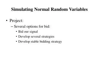
Simulating Normal Random Variables • Project: • Several options for bid: (1) Bid our signal (2) Develop several strategies (3) Develop stable bidding strategy
Simulating Normal Random Variables • Project: • Bidding the geologist’s signal is a bad idea • Leads to an average loss of approx. $21.7 million • What should be done?
Simulating Normal Random Variables • Project: • Create a simulation of 10000 auctions including all companies (use NORMINV) on a new worksheet • Find maximum error for each auction (represented by the variable C) • Find average of 10000 maximum values: E(C)
Simulating Normal Random Variables • Project:
Simulating Normal Random Variables • Project: • The average of the 10000 maximum values is called the “Winner’s Curse” • Defined as the average amount the winner of the auction would overbid by bidding their signal
Simulating Normal Random Variables • Project: • “First Plan” for a reasonable profit is to subtract E(C) from the geologist’s signal • This ensures that the winning company would break even on average
Simulating Normal Random Variables • Project: • This plan would not be reasonable, since the goal of a company is to make a fair and reasonable profit • To find a better strategy, find the gap between 1st place company and 2nd place company
Simulating Normal Random Variables • Project: • The monetary gap between 1st and 2nd is a wasted addition to the amount bid • The 1st place company must only outbid the 2nd place company by $0.01
Simulating Normal Random Variables • Project: • Find the value of the 2nd place company for each of the 10000 sample auctions (use LARGE function) • Once the 2nd place values are found, find the difference between 1st and 2nd (represented by variable B)
Simulating Normal Random Variables • Project: • For 10000 differences, find the average: E(B) • The average difference between 1st and 2nd place is called the “Winner’s Blessing” • Find 10 samples of E(C) and E(B) and average them
Simulating Normal Random Variables • Project:
Simulating Normal Random Variables • Project: • “Second Plan” ensures the winner of making a profit on average • Average profit is equal to E(B) • Strategy is not stable
Simulating Normal Random Variables • Project: • Remember that every company uses the same techniques to arrive at curse and blessing values • One company could decide to deviate from subtracting both the “Winner’s Curse” and the “Winner’s Blessing”
Simulating Normal Random Variables • Project: • Assume E(C) = $22.5 million and E(B) = $5.8 million • A company could decide to subtract $22.5 million and subtract $3.0 million (trying to outbid a company with a starting value higher than theirs)
Simulating Normal Random Variables • Project: • Ex: Company A: Signal $100 million (1st place) Company B: Signal $99 million (2nd place)
Simulating Normal Random Variables • Project: • Ex: Company A subtracts ($22.5 M and $5.8 M) leaving a bid of $71.7 million. Company B subtracts ($22.5 M and $3.0 M) deviating from a plan to subtract curse and blessing fully. This leaves a bid of $73.5 million.
Simulating Normal Random Variables • Project: • This process could continue endlessly • Find a stable bidding strategy • A stable bidding strategy means that any deviation from the suggested bid would not be beneficial over a large number of trials
Simulating Normal Random Variables • Project: • Stable bidding strategy has 2 steps (1) Find a trend line to predict a fair and reasonable adjustment amount if other companies subtract both E(C) and E(B). ($22.5 + $5.8 in millions) (2) Use the adjustment value in the Excel file Auction Equilibrium.xls to find a stable adjustment
Simulating Normal Random Variables • Project: • Create a new worksheet that calculates the errors for the 10000 simulated auctions minus 28.3 (error – (curse + blessing)) for all other companies • For your company (company 1), take the errors for the 10000 simulated auctions minus several different values (start around an adjustment of 13 and continue until an adjustment of around 31
Simulating Normal Random Variables • Project: • Find the maximum value (representing a winning company) • A negative maximum means that the winning company’s bid was below the proven value (making positive profit) • A positive maximum means that the winning company’s bid was above the proven value (company incurs a loss)
Simulating Normal Random Variables • Project: • Determine if company 1 (our company) wins each auction by using an IF statement • Determine how much profit the company would make by using IF statements
Simulating Normal Random Variables • Project: • Determine the probability of company 1 winning using COUNTIF, average extra profit, and the expected value of the adjustment • Determine the probability of every other company winning using COUNTIF, average extra profit, and the expected value of the adjustment
Simulating Normal Random Variables • Project: • Run the simulation several times to ensure accuracy • Average the results from several simulations • Record the results for adjustment (13, 15, 17, …, 31) and the expected values received
Simulating Normal Random Variables • Project: • Plot the points on a graph (x-axis will be adjustment values, y-axis will be expected value) • Fit a polynomial trend line of order 4 through the points • Estimate the maximum point (want a reasonable x-value) • This tells us how much we might want to subtract from estimate
Simulating Normal Random Variables • Project:
Simulating Normal Random Variables • Project:
Simulating Normal Random Variables • Project: • The peak is around x = 21 with y = 0.53
Simulating Normal Random Variables • Project: • The peak is around x = 21 with y = 0.53 • This means that a company should subtract approximately $21 million from their signal and receive an average of $0.53 million profit per auction