Download
1 / 53
540 likes | 863 Views
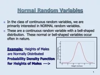
NORMAL RANDOM VARIABLES and why anyone cares. Sections 4.8-4.10. Normal Random Variables: Origin.

E N D
NORMAL RANDOM VARIABLESand why anyone cares Sections 4.8-4.10 Probability and Statistics for Teachers, Math 507, Lecture 11
Normal Random Variables: Origin • Abraham DeMoivre introduced the normal distribution in 1733 as a way of approximating binomial probabilities. The normal distribution is also known as the Gaussian distribution (ostensibly because Gauss studied its properties so extensively) and the bell curve (because of the shape of its pdf). Probability and Statistics for Teachers, Math 507, Lecture 11
Normal Random Variables: Origin • The normal distribution has turned out to be important as a model in its own right. In particular the Central Limit Theorem guarantees that as you take large enough samples from any random variable and average them, the averages tend toward a normal distribution. Probability and Statistics for Teachers, Math 507, Lecture 11
Normal Random Variables: Definition • We say that the random variable X has a normal distribution with parameters and 2, and we write X~normal(,2) if X has pdf Probability and Statistics for Teachers, Math 507, Lecture 11
Normal Random Variables: Definition • Note, in particular, that the range of X is the whole real line. The shape of this pdf is that of a mound or bell with its high point at (which turns out to be the mean of X). The mound is a narrow tall spike if 2 (which turns out to be the variance) is small. It is a broad low bump if 2 is large. Probability and Statistics for Teachers, Math 507, Lecture 11
Normal Random Variables: Definition • For instance, here is the graph of the pdf for =2.5 and 2=0.01. Probability and Statistics for Teachers, Math 507, Lecture 11
Normal Random Variables: Definition • And here is the graph of the pdf for =0 and 2=1. This is known as the standard normal random variable, commonly denoted by Z. Probability and Statistics for Teachers, Math 507, Lecture 11
Normal Random Variables: Definition • Neither of these looks very bell-like. The easiest way to get the typical bell-shaped curve is to use different scales on the axes. Here is the graph of Z again with different axes. Probability and Statistics for Teachers, Math 507, Lecture 11
Normal Random Variables: Expectation • Expectation: The expected value of X~normal(,2) is . This is Theorem 4.11 in the text. It follows directly from the definition of E(X), but it requires an algebraic trick and the fact that the integral of an odd function over an interval symmetric about the origin is always zero. Probability and Statistics for Teachers, Math 507, Lecture 11
Normal Random Variables: Variance • Variance: Similarly the variance of X~normal(,2) is 2. Again this follows directly from the definition of Var(X) after a change of variables and integration by parts. Probability and Statistics for Teachers, Math 507, Lecture 11
Normal Random Variables: CDF • By definition the cumulative distribution function of X~normal(,2) is Probability and Statistics for Teachers, Math 507, Lecture 11
Normal Random Variables: CDF • This function, however, while nicely behaved (continuous, indeed smooth) is not a simple function. It is not expressible by a finite combination of the familiar functions (polynomial, trig, exponential, log, algebraic) through addition, subtraction, multiplication, division, and composition. To find values of the cdf we must approximate them. In practice this means we consult a table of values of the cdf. Probability and Statistics for Teachers, Math 507, Lecture 11
Normal Random Variables: CDF • Offhand it appears we need a different table for every choice of values for and 2. It turns out, however, that every linear function of a normal random variable is also normal. In particular if X~normal(,2), and Z=(X‑)/, then Z~normal(0,1). Thus knowing the cdf for Z suffices to find it for every normal random variable. Here is the proof: Probability and Statistics for Teachers, Math 507, Lecture 11
Normal Random Variables: CDF • Let F denote the cdf of Z. Then Probability and Statistics for Teachers, Math 507, Lecture 11
Normal Random Variables: CDF • It is conventional to denote the cdf of Z by rather than F. So if X~normal(,2), we can find values of its cdf by transforming X into a standard normal random variable and then looking the values up. That is Probability and Statistics for Teachers, Math 507, Lecture 11
Standard Normal Random Variables • Definition: The random variable Z~normal(0,1) is called the standard normal random variable. • Evaluation of Probabilities: Tables of the values of (z), the cdf of Z, are readily available. The table on p. 114 of our text is typical. It lists (z) for all values of z between –3.09 and +3.09, in increments of 0.01. To look up (z) for a particular value of z, find the units and tenths digits of z in the left hand column and find the hundredths digit of z across the top row. The row and column intersect at the value of (z). For instance (1.37)=0.9147 . Probability and Statistics for Teachers, Math 507, Lecture 11
Standard Normal Random Variables • With this table we can easily compute P(Z a)=(a), P(a Z b)=(b)-(a) and P(Z b)=1-(b). • Note that many freshman statistics texts give tables of P(0<Z<z) for positive z only instead of a table of the cdf. This serves the same purpose, but the technical details of computing probabilities differ a bit. To avoid embarrassment when teaching this subject, be sure to practice with whatever table is in your text before you try to “wing it” with an example in front of class. Of course some calculators (the TI-83 in particular, I believe) will calculate values of the cdf and pdf of standard normal random variables (and other random variables as far as that goes). Probability and Statistics for Teachers, Math 507, Lecture 11
Comparison To Chebyshev • If X~normal(,2), and h>0, then by Chebyshev’s Theorem This says X has a probability of at least 0 of falling within one standard deviation of its mean, at least ¾=75% of falling within two standard deviations, and at least 8/9=88.9% of falling within three standard deviations. Probability and Statistics for Teachers, Math 507, Lecture 11
Comparison To Chebyshev • These lower bounds are far from sharp for normal random variables. We can compute the actual probability of normal X falling within one standard deviation of its mean as Probability and Statistics for Teachers, Math 507, Lecture 11
Comparison To Chebyshev • Similarly X~normal(,2) has probability 0.9544 of falling within two standard deviations of its mean and probability 0.9974 of falling within three standard deviations of its mean. Note that these values are much higher than the lower bounds from Chebyshev’s theorem. It is worth putting in long term memory that a normal random variable falls within one, two, or three, standard deviations of its mean with probabilities 68%, 95%, and 99.7% respectively. The same is true about approximate percentages of data falling within one, two, and three standard deviations of the mean when the data is drawn from a normally-distributed population. Probability and Statistics for Teachers, Math 507, Lecture 11
Examples: Women’s Heights • Some data suggests that the mean height of female college students is roughly normally distributed with mean 65 inches and standard deviation 2.5 inches. Approximately what percentage of female college students are over 70 inches tall? Probability and Statistics for Teachers, Math 507, Lecture 11
Examples: Women’s Heights • Let X be the height of a randomly selected female college student. Then X~normal(65”,6.25in2). Then we want P(X>70”). We compute this as follows: Just over 2% of female college students are over 70” tall. Probability and Statistics for Teachers, Math 507, Lecture 11
Examples: SAT Scores • If X is a random variable, then the qth percentile of X is a number xq such that F(xq)=q/100. In other words it is the number such that X has probability q% of being less than it. For example, the 25th percentile x25 has property that F(x25)=0.25=25%. It is common to call the 25th percentile the lower quartile, the 50th percentile the median, and the 75th percentile the upper quartile. Probability and Statistics for Teachers, Math 507, Lecture 11
Examples: SAT Scores • If SAT scores are normally distributed with mean 500 and standard deviation 100, what percentile is a score of 650? The SAT scores are a random variable X~normal(500,1002). Then Probability and Statistics for Teachers, Math 507, Lecture 11
Examples: SAT Scores • What percentile is a score of 300? Here we compute F(300)=(‑2)=0.0228, the 2.28th percentile. • What is the 90th percentile of the SAT scores? We want x90 such that F(x90)=0.90. This is equivalent to (( x90 –500)/100)=0.90. We use the standard normal table backward to find that a suitable z is approximately 1.28 (since (1.28)=0.8997). Solving (x90 –500)/100=1.28, we get x90=628. Probability and Statistics for Teachers, Math 507, Lecture 11
Approximation Formula for • The text mentions a rational approximation formula for (z) that you can program into your calculator. In practice you can probably get access to a TI-83 or other calculator with built in. Also the major spreadsheet programs have many of the pdfs, cdfs, and inverse cdfs (equivalent to using the table backwards) as built-in functions. Indeed I produced all of the graphs in the following section using the binomdist and normdist functions in Excel. Probability and Statistics for Teachers, Math 507, Lecture 11
DeMoivre-Laplace Theorem: Approximating Binomial Distributions by Normal • Visual Normality of Binomial Distributions: Under many circumstances the binomial distribution has much the shape of a normal distribution. This is easy to see by graphing the pdf of a binomial distribution as a histogram. Note that in such a histogram (as in a continuous pdf) the area of each block is the probability of the corresponding value of X and the total of the areas is 1. Thus we can treat the histogram as a continuous pdf (a step function). Probability and Statistics for Teachers, Math 507, Lecture 11
DeMoivre-Laplace Theorem • For p=0.5 as n increases: On p.117 we see the histogram for X~binomial(n,0.5) as n increases from 10 to 100. Notice how the graph is roughly normal at every step but becomes flatter and more spread out as n increases. • For small n when p is not extreme: On p. 118 we see the histograms for X~binomial(n,p) with n between 1 and 8, and p between 1/8 and 7/8. Extreme values of p lead to highly non-normal histograms for these low values of n. But p=1/2 leads to roughly normal histograms throughout, and by n=8 even the histograms for p=1/4 and p=3/4 are starting to take on a bell shape. Probability and Statistics for Teachers, Math 507, Lecture 11
DeMoivre-Laplace Theorem • For more p when n becomes large: On p. 119 we see the histograms for X~binomial(100,p) for p between 10% and 90%. The histograms are roughly bell shaped throughout, spikier at the extremes and more spread out near the middle. • Here is a comparison of four histograms for X~binomial(100,p), for p= 0.5, 0.75, 0.10, and 0.98. Note that the graph grows taller, narrower, and less symmetric as p departs farther from 0.50, finally growing distinctly non-normal at p=0.98. Probability and Statistics for Teachers, Math 507, Lecture 11
Probability and Statistics for Teachers, Math 507, Lecture 11
DeMoivre-Laplace Theorem • The following four graphs compare each of the previous histogram (now as line graphs in blue) to the normal curves (in purple) with the same means and standard deviations. Note how the match is essentially perfect for p=0.50 and grows progressively worse as p moves toward the extreme values. In the graph for p=0.98 the masked portion at the right indicates the values above 100. The binomial random variable cannot take on those values, but notice how much area lies below the normal curve in that range. This indicates badness of fit between the variables. Probability and Statistics for Teachers, Math 507, Lecture 11
Probability and Statistics for Teachers, Math 507, Lecture 11
Probability and Statistics for Teachers, Math 507, Lecture 11
Probability and Statistics for Teachers, Math 507, Lecture 11
Probability and Statistics for Teachers, Math 507, Lecture 11
DeMoivre-Laplace Theorem • This suggests that for n sufficiently large the distributions of X~binomial(n,p) and Y~normal(np,npq) are approximately equal. But since is normal, then should be approximately standard normal. This turns out to be the case. Probability and Statistics for Teachers, Math 507, Lecture 11
DeMoivre-Laplace Theorem • Theorem 4.13 (DeMoivre-Laplace): If X~binomial(n,p), then for all real numbers Probability and Statistics for Teachers, Math 507, Lecture 11
DeMoivre-Laplace Theorem • This is a special case of the Central Limit Theorem. It says that if you draw n samples from a (any!) random variable with mean and variance 2, then as n increases, the average of the n values has an approximately normal distribution with mean and variance 2/n. Probability and Statistics for Teachers, Math 507, Lecture 11
The Continuity Correction • Suppose X~binomial(n,p) and Y~normal(np,npq). The above discussion suggests approximating P(X b) by P(Y b). In the histogram for X, however, each bar — in particular the bar for X=b — has a width of one, stretching from b1/2 to b+1/2. Thus we get a better approximation by using P(Y b+1/2) or more properly by Probability and Statistics for Teachers, Math 507, Lecture 11
The Continuity Correction • Similarly we do best to approximate P(a X b) by P(a1/2 Y b+1/2) or more properly by Probability and Statistics for Teachers, Math 507, Lecture 11
The Continuity Correction • This modification is known as the correction for continuity. The following graph illustrates why it helps, superimposing the blue bars of the binomial histogram on the red area under the normal curve. Probability and Statistics for Teachers, Math 507, Lecture 11
Probability and Statistics for Teachers, Math 507, Lecture 11
Criteria for Approximating the Binomial by the Normal • How do we decide when the normal is a good approximation to the binomial? The text gives the guideline that 3 or equivalently that n 9/(pq). The table in the text shows the appropriate values of n for various choices of p. Note that n stays modest unless p is extreme. Other authors suggest using the criterion that 0 -3<+3<n. The point of this criterion is that all values of the normal curve within 3 standard deviations of the mean should lie within the range of the binomial random variable under discussion (the condition violated by X~binomial(100.0.98) above). Probability and Statistics for Teachers, Math 507, Lecture 11
Examples of Approximating the Binomial by the Normal • Tossing a coin 25 times • If you toss a fair coin 25 times, what is the probability of getting exactly 12 heads. Here we have X~binomial(25,0.5). Based on the discussion at the bottom of p. 122, this n is large enough to support a normal approximation. We calculate • This answer is correct to three decimal places. Probability and Statistics for Teachers, Math 507, Lecture 11
Examples of Approximating the Binomial by the Normal • Tossing a coin 25 times • To approximate the probability P(X 18), we use Probability and Statistics for Teachers, Math 507, Lecture 11
Examples of Approximating the Binomial by the Normal • A binomial probability with small p • If X~binomial(1000, 0.01), approximate P(X 3). Here we see n>9/(pq) since n=1000 and 9/(pq) is about 909, so a normal approximation is appropriate. • Applying the correction for continuity, we calculate Probability and Statistics for Teachers, Math 507, Lecture 11
Examples of Approximating the Binomial by the Normal • A binomial probability with small p • Note that we rounded the Z value to two decimal places since that is what the table for contains. Also note how much simpler this approach is than calculating the exact value using the binomial distribution. For instance we avoid calculating the 998th power of 0.99. Probability and Statistics for Teachers, Math 507, Lecture 11
Examples of Approximating the Binomial by the Normal • A hypothesis test for coin flips • A supposedly fair coin turns up heads 62 times in 100 flips. Does this provide evidence of bias toward heads at the 1% significance level? If X is the number of heads, then under the null hypothesis (fair coin) X~binomial(100,0.5). What is the probability of getting data as contradictory to the null hypothesis (or more so) as we actually got? If that probability is under 1%, we reject the null hypothesis. Probability and Statistics for Teachers, Math 507, Lecture 11
Examples of Approximating the Binomial by the Normal • A hypothesis test for coin flips • We need P(X 62). Since 9/(pq)=36 and n=100>36, we may use a normal approximation. Thus • Since this probability exceeds (although just barely, at 1.07%) our proposed significance level of 1%, we do not reject the null hypothesis. We remain unconvinced that the coin is biased toward heads. (This is not to say that we are convinced that it is not biased.) Probability and Statistics for Teachers, Math 507, Lecture 11
Examples of Approximating the Binomial by the Normal • A hypothesis test for army recruiting • Suppose the army claims to have only 10% of recruits without a high school diploma. A random sample of 625 recruits includes 75 without a diploma. Does this provide sufficient evidence at the 5% significance level that the army’s claim is incorrect? Under the null hypothesis (i.e., the army’s claim is correct), we have X~binomial(625,0.10), where X is the number of recruits in the sample without high school diplomas. We note that 9/(pq)=100 and n>100, so a normal approximation is appropriate. Probability and Statistics for Teachers, Math 507, Lecture 11