Download
1 / 54
550 likes | 1.25k Views
Addition of Independent Normal Random Variables . Theorem 1 : Let X and Y be two independent random variables with the N ( , 2 ) distribution. Then, is N (2 , 2 2 ) . Proof : . Subtraction of Independent Normal Random Variables. Theorem 2 :

E N D
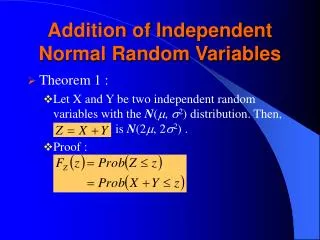
Addition of Independent Normal Random Variables • Theorem 1 : • Let X and Y be two independent random variables with the N(, 2) distribution. Then, is N(2, 22) . • Proof :
Subtraction of Independent Normal Random Variables • Theorem 2 : • Let X and Y be two independent random variables with the N(, 2) distribution. Then, is N(0, 22) . • Proof : • Similar to the proof of Theorem 1.
Generalization of Theorem 1 • Let X1, X2, ……, Xn be n mutually independent normal random variables with means μ1, μ2, …, μn and variances , respectively. • Then, is .
Chi-Square Distribution with High Degree of Freedom • Assume that X1, X2, ……, Xkare k independent random variables and each Xiis N(0, 1). • Then, the random variable Z defined by is called a chi-square random variable with degree of freedom =k and is denoted by .
Example of Chi-Square Distribution with Degree of Freedom = 2 • Let X,Y be two independent standard normal random variables, and Z = X2 + Y2.
Example of Chi-Square Distribution with Degree of Freedom = 3 • Let X,Y,Z be three independent standard normal random variables, and W = X2 +Y2 + Z2.
Note that, The surface area of a sphere in the k-dimensional vector space is
Moment-Generating Function of the Distribution • The moment-generating function of a distribution with p.d.f f(x) is defined to be • Note that
Theorem: The moment-generating function Mk(z) of is Proof: since the p.d.f of is only defined in [0,∞) we now consider two cases: (1) k=2h (2) k=2h+1
By applying the same technique repetitively we get we can prove that for both k=2h and k=2h+1 cases,
Estimation of the Expected Value of a Normal Distribution • Let X be a normal random variable with unknown μ and σ2. • Assume that we take n random samples of X and want to estimate μ andσ2 of X based on the samples. • Let denote an estimation of μ. Then, the likelihood function of n samples is
~continues • Therefore, is a maximum likelihood estimator of μ.
~continues • Let X1, X2, … Xn be the random variables corresponding to sampling X n times. Since is called an unbiased estimator of μ. Furthermore, since ,the confidence interval of μ approaches 0 , as n →∞, provided that is used as the estimator of μ. The confidence interval of μ is
That is the confidence interval of S2 approaches 0 as n→∞, provided that S2is used as the estimator of σ2
An Important Observation There are more general situation in which a degree of freedom of chi-square distributions is lost for each parameter estimated.
Test of Statistical Hypotheses • The goal is to prove that a hypothesis H0 does not hold in the statistical sense. • We first assume that H0 holds and design a statistical experiment based on the assumption. • The probability that we reject H0 when H0 actually holds is called the significance level of the test. Typically, we use to denote the significance level.
An Example of Statistical Tests • We want to prove that a coin is biased. • We make the following hypothesis “The coin is unbiased”. • We design an experiment that is to toss the coin n times and we claim the coin is biased, i.e. rejecting the hypothesis, if we observe either one side is up k times or more, where k > ½ n.
~continues • Let X be the random variable corresponding the number of times that one particular side is up in n tosses. • Under the hypothesis “The coin is unbiased”, approaches N(0, 1). • The significance level of the test is
~continues • Assume that we want to achieve a significance level of 0.05 and we toss the coin 100 times. Since , • Assume that we want to achieve the same level of significance and we toss the coin 1000 times.Then,
Test of Equality of Several Means • Assume that we conduct k experiments and all the outcomes of the k experiments are normally distributed with a common variance. Our concern now is whether these k normal distributions, N(1,2), N(2,2),…, N(k,2), have a common mean, i.e. 1= 2=…= k.
One application of this type of statistical tests is to determine whether the students in several schools have similar academic performance. • The hypothesis of the test is . 1= 2=…= k.
Let ni denote the number of smaples that we take from distribution N(i,2). As a result, we have the following radom variables: X11, X12,…, X1n1 : samples from N(1,2). X21, X22,…, X2n2 : samples from N(2,2). … … … … … Xk1, Xk2,…, Xknk : samples from N(k,2).
Chi-Square Test of Independence for 2x2 Contingence Tables • Assume a doctor wants to determine whether a new treatment can further improve the condition of liver cancer patients. Following is the data the doctor has collected after a certain period of clinical trials.
~continues • The improvement rate when the new treatment is applied is 0.85 and the rate is 0.77 when the conventional treatment is not applied. So, we observe difference. However, is the difference statistically significant? • To conduct the statistical test, we set the following hypothesis H0 :“ The effectiveness of the new treatment is the same as that of the conventional treatment.”
~continues • Under H0, the two rows of the 2x2 contingence table corresponds to two independent binomial experiments, denoted by X1and X2 , respectively. • Define parameters as follows.
Let Y1, Y2, …, Yn1 be n1 samples taken from a normal distribution N( p, p(1-p) ). Then, is
Therefore, the distribution of Z1 approaches that of . Similarly, let be samples taken from a normal distribution N( p, p(1-p)). Then the distribution of Z2 approaches that of • Since and are samples from a statisctical test of two means, is , where
Since the distributions of Z1 and Z2 approach those of and , respectively, approaches . is an estimator of the mean of Yi and Wj, which is p. Therefore, if we use as the estimator, then we have approaches
According to our previous observation, we have In conclusion,
~continues • Applying the data in our example to the equation that we just desired, we get • Therefore, we have over 97.5% confidence that the new treatment is more effective than the conventional treatment.
~continues • On the other hand, if the number of patients that have been involved in the clinical trials is reduced by one half, then we get • Therefore, we have less than 90% confidence when claiming that the new treatment is more effective than the conventional treatment.
A Remark on the Chi-Square Test of independence • The chi-square test of independence only tell us whether two factors are dependent or not. It does not tell us whether they are positively correlated or negatively correlated. • For example, the following data set gives us exactly identical chi-square value as our previous example.
Measure of Correlation • Correlation (A,B) = P(A&B) / P(A)P(B) = P(A|B)P(B) = P(B|A)P(A). • Correlation(a,b) = 1 implies that A and B are independent. • Correlation(a,b) > 1 implies that A and B are positively correlated. • Correlation(a,b) < 1 implies that A and B are negatively correlated.
Generalizing the Chi-Square Test of Independence • Given a 32 contingency table as follows. • Let Z1, Z2 and Z3 be the three random variables corresponding to the experiments defined by the three rows in the contingency table.
The Chi-Square Statistic for Multinomial Experiments • Given the 32 contingency table . • We can regard the table as the outcomes of 2 independent multinomial experiments.