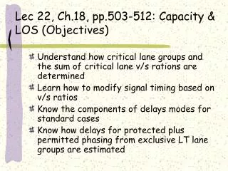
Lec 22, Ch.18, pp.503-512: Capacity & LOS (Objectives)

1. Lec 22, Ch.18, pp.503-512: Capacity & LOS (Objectives) • Understand how critical lane groups and the sum of critical lane v/s rations are determined • Learn how to modify signal timing based on v/s ratios • Know the components of delays modes for standard cases • Know how delays for protected plus permitted phasing from exclusive LT lane groups are estimated

2. What we discuss in class today… • Steps for determining critical lane groups and the sum of critical lane v/s ratios • Method to determine lane group capacities and v/c ratios • Method to modify signal timing based on v/s rations • Delay models for standard cases • Delay models for protected plus permitted phasing from exclusive LT lane groups • Issues relating to the analysis of actuated signals

3. HCM-way of determining lane groups and the sum of critical lane group v/s ratios • In a simple signal timing method, critical lane groups were determined by comparing adjusted per lane flows in each lane group using a ring diagram. • In the 2000 HCM, per-lane flows cannot be compared because we have lane group flows. So, we use v/s ratios to determine critical lane groups. • Once the v/s is computed (the outcomes of Module 2 and 3 of the 2000 HCM), v/s is used to determine critical lane groups and a ring diagram is again used.

4. Example of finding critical lane groups using v/s ratios (p.504) tL takes place.

5. Example of finding critical lane groups using v/s ratios (p.504) – cont. This indicates the proportion of real time that must be devoted to effective green. In this case 90% of the cycle. Conversely, 1 – 0.9 = 0.1 is available for lost times. Hence in this example, In general, Webster model,

6. Determining lane group capacities and v/c ratios • Determining lane group capacities and v/c ratios is straight forward. • Capacity for lane group i : • v/c ratio for lane group i , X: • The critical v/c ratio for the intersection can be found using Equation 18-4 in page 470: Note that

7. Modifying signal timing based on v/s ratios • After v/s ratios are computed, we may need to make adjustments – either reallocation of green time, modifying cycle length, or modifying the intersection layout. For the first two cases, v/s rations can be used to reduce the amount of trial-and-error computations. First, we solve Eq. 18-4 for C: When Xc = 1.0, it is like C equation for simple signal timing. • Suppose sum(v/s) = 0.9, and we desire to achieve Xc = 0.95. What would be the cycle length to achieve this for the problem in Figure 18-18? Xc = 0.95 cannot be achieved in this case. C = 171 sec is too long.

8. Modifying signal timing based on v/s ratios (cont) • C needs to be contained within the common cycle lengths. Typically C = 120 sec is the maximum cycle length accepted. Hence, Where, gi = C – L. With sum(v/s) = 0.90 and C = 120 sec, Xc = 0.973 is the minimum that can be achieved. Once C is determined, we can compute new effective greens,then new actual greens for the next trial-and-error analysis.

9. LOS module • This is the last step—estimating average individual stopped delays for each lane group. 1. Delay models for standard cases (for permitted or protected or compound phasing phasing from a shared lane group): (Eq. F16.1, p.16-144)

10. LOS module (cont) 2. Delay models for protected plus permitted phasing from exclusive LT lane groups • “it should be noted that compound phasing is not generally used when more than one exclusive lane is present.”  What this confusing statement wants to say is “when double exclusive LT lanes exist, compound phasing is not used. Protected LT phase is always used for double exclusive LT arrangement for safety.” • The effect of compound phasing applies only to the uniform delay component. It is adjusted to reflect varying arrival and departure patterns. Five different cases may arise as you see in the next slide.

11. Leading LT phase Lagging LT phase Permitted Protected

12. Determining the case Capacity (max service flow during g) Total approach volumes during r + g qa = approach flow rate, vph

13. Uniform delay formulas d1 = [0.5/ Total arrival volume during a cycle (because we are computing average control delay per vehicle) qa g Note that this g and gu do not have to be their interval values. Simply, they are the time needed to clear the queues. Area = total delay (veh.sec) sp g qa sp Qa r g

14. A close look at the delay for Case 1 Note that the delay computed from this diagram is approach delay. Divide it by 1.3 to get stopped delay. B A A Area = (1/2)rQa Hence, 0.38rQa tc B To find the area of B, we need to find tc. sp*tc = Qa + qa*tc tc = Qa/(sp – qa) Area = (1/2)Qa*Qa/(sp – qa) = (1/2)Qa2/(sp – qa) Hence, 0.38Qa2/(sp – qa)

15. Numerical example for multiple time periods See page 16-146 in Appendix F Use the overhead projector…