Scientific Presentation for: ACM-Ice-Reading (variational synergetic ice retrieval)

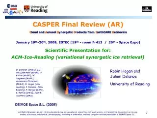
1. CASPER Final Review (AR)Cloud and Aerosol Synergetic Products from EarthCARE RetrievalsJanuary 19th-20th, 2009, ESTEC [19th - room Fr413 / 20th - Space Expo] Scientific Presentation for: ACM-Ice-Reading (variational synergetic ice retrieval) D. Donovan (KNMI), G.J. van Zadelhoff‘ (KNMI) P. Kollias (McGill), W. Szyrmer (McGill), Aleksandra Tatarevic (McGill), R. Hogan (Univ. reading), J. Delanoe (Univ. Reading), F. Berger (DWD), K. Barfus (DWD), Juan-R. Acarreta (DMS) Robin Hogan and Julien Delanoe University of Reading DEIMOS Space S.L. (2009)

2. Overview • Introduction • Summary of achievements in Casper • Overview of synergy products, need for target classification • CASPER Algorithm: ACM-Ice-Reading (including AC-Ice-Reading) • Why this algorithm is needed ? • Input Data and Product Definition • Theoretical description • Summary of the performance and error analysis • Verification and Validation • “Blind-test” cases using aircraft data • ECSIM cases • Application of a similar algorithm to CloudSat, CALIPSO and MODIS • Conclusions • Generalizing to “unified” synergy algorithm • Recommendations for necessary post-Casper work

3. Summary of achievements • Identified the synergy products required by EarthCARE • Reviewed the relevant literature for each of them (PARD) • Prioritized future work on synergy algorithms for EarthCARE • Described a retrieval algorithm for ice clouds that uses radar, HSRL lidar and infrared radiances (ATBD) • Developed the code for the algorithm • Integrated it into ECSIM • Tested the code on simulated data • Applied a similar algorithm (simple backscatter rather than HSRL) to a month of CloudSat/CALIPSO/MODIS data

4. Synergy (Level 2b) overview • Target classification • Radar-lidar target classification • Two-instrument algorithms • Various combinations of radar (Z, v), lidar (backscatter, HSRL), MSI (IR, solar)… • To estimate ice, liquid, aerosol, precipitation properties • Too many combinations possible – need to be selective • Three-instrument algorithms • Needs variational framework • Higher level products • L2b-2D Cloud fraction, overlap, mean water content and inhomogeneity on pseudo-model grid

5. Reading contribution to Casper Implemented in Casper (ATBD) Planned in Casper (PARD)

6. Target Classification product • Importance: MANDATORY • Classification essential to facilitate synergetic algorithms • Also useful to provide one file from which subsequent algorithms could run by regridding, storing errors etc. • Maturity: NOVEL/MATURE • This work has been carried out on ground-based radar and lidar data • Application to CloudSat/CALIPSO is ongoing but less mature • Wang & Sassen (2001) designed CloudSat 2B-CLDCLASS • Attempt to match traditional classification of “stratocu”, “altostratus” etc. • But subsequent algorithms actually want to know • Target phase (liquid/ice) and where we can’t be sure • Whether cloud or precipitation • Details: Hail/graupel, melting ice, warm/”cold” rain? • Other targets: aerosol, insects, molecular • Co-existence of the above target types

7. Ground-based classification Ground-based cloud radar observations from Chilbolton • Example of target classification during the “Cloudnet” project • In this case the classes are: ice, liquid cloud, drizzle/rain and aerosol

8. CloudSat/CALIPSO This is an example of how such a product might look Priority for development after CASPER Cloudsat radar CALIPSO lidar Insects Aerosol Rain Supercooled liquid cloud Warm liquid cloud Ice and supercooled liquid Ice Clear No ice/rain but possibly liquid Ground Preliminary target classification

9. Radar-Lidar-MSI ice cloud product • Why is this product required? • Ice clouds an important component of the radiation budget of the earth, and their properties still vary widely in climate models • A lot is known on how to combine radar and lidar in synergy, and indeed much of the preparatory work has been carried out • By adding MSI information the profile of cloud properties should more consistent with the broadband radiation measurements, which is a key mission requirement • This product should be the first “official” global radar-lidar retrieval of ice cloud properties, particularly effective radius • Therefore this product is a key EarthCARE output and is Mandatory • Radar-Lidar (AC-Ice-Reading) version is Mature • Radar-Lidar-Radiometer (ACM-Ice-Reading) version is Novel

10. Input data required • Platform and orbit parameters • time(t), longitude(t), latitude(t), altitude(t), height(t,z) ... • Instrument characteristics • lidar_div, lidar_fov, C_lid(t) • Measurements • Z(t, z), bscat_Mie(t, z), bscat_Ray(t, z), radiance(t, l) • Measurement errors • Standard error in each of the input data • Cloud mask • mask_radar(t, z), mask_lidar(t, z), cloud_phase(t, z) • Met and surface data (ECMWF) • temperature(t, z), pressure(t, z), q(t, z), ozone(t, z) • surf_pressure(t), skin_temperature(t), surf_emissivity(t) • Note that these are as in the KNMI “merged file”

11. Product definition • Platform and orbit parameters • Repeated from the input data • Directly retrieved variables • Extinction (t, z), N0* (t, z), lidar_ratio (t, z) • Variables derived from retrieved variables • IWC (t, z), re (t, z), optical depth (t) • Forward modelled variables at final iteration • Z_fwd (t,z), bscat_Mie_fwd (t,z), bscat_Ray_fwd (t,z), radiance_fwd(t,l) • Measures of convergence • n_iterations (t), chi_squared (t, iteration) • Status flags • retrieval_flag (t, z), instrument_flag(t, z), radiance_flag(t) • Error standard deviations • ln_extinction_err (t, z), ln_N0*_err(t, z), ln_lidar_ratio_err(t, z) • ln_IWC_err (t, z), ln_effective_radius_err(t, z), optical_depth_err (t)

12. Previous 2-instrument algorithms • Various combinations of instruments similar to those on EarthCARE have been tried for ice clouds before • Lidar and radar definitely the most promising! • Radar ZD6, lidar b’D2 so the combination provides particle size

13. Radar-lidar ice algorithm history • Don’t correct lidar for attenuation: Intrieri et al. (1993) • Limited to very thin clouds; lidar ratio must be assumed • Invert lidar separately: Mace et al. (1998), Wang & Sassen (2002), Okamoto et al. (2003) • Extinction error increases into cloud due to assumed lidar ratio • Optimal estimation but lidar inverted separately: Mitrescu et al. (2005) • Same lidar errors as Wang & Sassen • Invert lidar with radar: Donovan & van Lammeren (2001), Tinel et al. (2005) • Lidar ratio is retrieved: much more accurate • Full optimal-estimation (=variational) approach: Delanoe & Hogan (2008) • Same strengths as Donovan & van Lammeren • Allows extra constraints/obs to be included, e.g. infrared radiances • Can blend into regions detected only by radar or lidar • Provides retrieval errors and error covariances • Exploit the HSRL channels when available (new in CASPER)

14. HSRL Mie channel HSRL Rayleigh channel Radar reflectivity Radiances Extinction coefficient Lidar ratio Ratio N0*/a0.6 Formulation of the problem • State vector • Retrieved variables • Observation vector • Elements may be missing

15. Synergetic retrieval framework Minimize cost function of the form: J = squared difference between observations and forward model + squared difference between state vector and a-priori + smoothness constraints New ray of data: define state vector x Use merged fileto specify variables describing ice cloud at each gate Radar model Radar reflectivity Lidar model Including HSRL channels and multiple scattering Radiance model IR channels Forward model Compare to observations Check for convergence Not converged Gauss-Newton iteration Derive a new state vector Converged Calculate errors and proceed to next ray of data

16. Why N0*/a0.6? • In-situ aircraft data show that N0*/a0.6 has temperature dependence that is independent of IWC • Therefore we have a good a-priori estimate to constrain the retrieval • Also assume vertical correlation to spread information in height, particularly to parts of the profile detected by only one instrument

17. Why N0*??? • We need to be able to forward model Z and other variables from x • Large scatter between extinction and Z implies 2D lookup-table is required • When normalized by N0*, there is a near-unique relationship between a/N0* and Z/N0* (as well as re, IWC/N0* etc.)

18. Lidar field-of-view (equivalent medium theorem allows forward scattering on the return journey to be neglected) Modelling HSRL with multiple scattering • Photon variance-covariance method • Hogan (Applied Optics 2006, JAS 2008) • As light propagates through a medium where size r » wavelength l, narrow-angle forward-scattering widens beam • Write down differential equations for • Total energy P • Positional variance • Directional variance • Covariance • E.g. z s r • Thus can calculate positional variance versus range z and hence the fraction of light remaining in field of view • Very efficient: time proportional to number of pixels squared • Modelling HSRL channels in CASPER: a straightforward modification • Particles and molecules already treated separately since molecules don’t have a forward-scattering lobe

19. Effect of errors on retrievals Partly taken from Hogan et al. (JTECH 2006)

20. No HSRL • Aircraft-observed ice size spectra used to generate pseudo-measurements (Hogan et al 2006 “blind test” case) • Note that the same lidar forward model (which includes multiple scattering) is used in generating the pseudo-measurements and in the retrieval • Lidar ratio S assumed constant in retrieval “Measurements” Retrievals

21. With HSRL • S free to vary with height (except for smoothness constraint) • Can reproduce features of true S • More accurate extinction where lidar has signal • Some noise from Rayleigh channel in retrieved S: need more smoothness “Measurements” Retrievals

22. ECSIM radar reflectivity ECSIM fractal cirrus case KNMI have run ECSIM using a cirrus cloud generated by the Hogan and Kew (2005) model ECSIM lidar Rayleigh channel ECSIM lidar Mie channel

23. ECSIM radar reflectivity ECSIM fractal cirrus case KNMI have run ECSIM using a cirrus cloud generated by the Hogan and Kew (2005) model At the final iteration, the variational scheme attempts to “forward model” the observations but without reproducing instrument noise Retrieval forward model ECSIM lidar Rayleigh channel ECSIM lidar Mie channel Retrieval forward model Retrieval forward model

24. Comparison with “truth” “True” ECSIM extinction coefficient Slightly poorer agreement than “blind-test” profiles, presumably because ECSIM instrument simulator different from forward model in the retrieval algorithm Retrieved extinction coefficient Retrieved effective radius Retrieved ice water content

25. …Add radiances to retrieval “True” ECSIM extinction coefficient Merits of radiances are inconclusive; HSRL already accurate, and forward-model errors may be important… Retrieved extinction coefficient Retrieved effective radius Retrieved ice water content

26. Lidar observations Radar observations CloudSat-CALIPSO-MODIS example 1000 km

27. Lidar observations Lidar forward model Radar observations Radar forward model CloudSat-CALIPSO-MODIS example

28. Extinction coefficient Ice water content Effective radius Radar-lidar retrieval Forward model MODIS 10.8-mm observations

29. Radiances matched by increasing extinction near cloud top …add infrared radiances Forward model MODIS 10.8-mm observations

30. Radar-lidar complementarity MODIS 11 micron channel Retrieved extinction (m-1) CloudSat radar Deep convection penetrated only by radar Height (km) CALIPSO lidar Cirrus detected only by lidar Height (km) Mid-level liquid clouds Time since start of orbit (s)

31. 1-month optical depth comparison Mean of all skies Mean of clouds CloudSat-CALIPSO MODIS • Mean optical depth from CloudSat-CALIPSO is lower than MODIS simply because CALIPSO detected many more optically thin clouds not seen by MODIS • Hence need to compare PDFs as well

32. First comparison with ECMWF log10(IWC[kg m-3])

33. Comparison with model IWC Global forecast model data extracted underneath A-Train A-Train ice water content averaged to model grid Met Office model lacks observed variability ECMWF model has artificial threshold for snow at around 10-4 kg m-3 A-Train Met Office ECMWF Temperature (°C) Temperature (°C)

34. Post-Casper work • Essential further work for ACM-Ice-Reading algorithm: • Verify that when one of the instruments is missing, algorithm will approximate existing two-instrument algorithms, e.g. Chiriaco et al. (lidar-MSI) • Check infrared forward model (e.g. against “RTTOV”) • Apply to real HSRL data and compare to in-situ “truth” • Broader outlook for synergy algorithms for EarthCARE • Develop “unified” algorithm to retrieve all species (ice cloud, liquid cloud, aerosols and precipitation) simultaneously; often several present in the same profile • Considerable work required to select best state vector etc.

35. General synergetic framework New ray of data: define state vector Use classification to specify variables describing each species at each gate • Ice:extinction coefficient and N0* • Liquid: liquid water content and number concentration • Rain: rain rate and mean drop diameter • Aerosol: extinction coefficient and particle size (Black) Ingredients delivered in Casper (Delanoe and Hogan JGR 2008) (Red) Ingredients remaining to be developed Radar model Including surface return and multiple scattering Lidar model Including HSRL channels and multiple scattering Radiance model Solar and IR channels Forward model Compare to observations Check for convergence Not converged Gauss-Newton iteration Derive a new state vector Converged Proceed to next ray of data

36. Components of liquid-cloud algorithm

37. Recommendations • Radar/lidar mis-pointing should be < 500 m, equivalent to RMS error in Z of 0.5 dB • Most two-instrument algorithms should be tested as limiting cases of a more general multi-instrument algorithm, covering EarthCARE in case of instrument failure • The target classification should be developed as a priority, and would include the measurements on the same grid, to facilitate synergetic algorithms • Level 2b-2D products should be produced: cloud fraction, overlap, etc., under EarthCARE but averaged to typical model resolution; satisfies a key mission requirement • A flexible optimal-estimation software library should be developed to facilitate implementation of synergetic algorithms, in particular the “best-estimate” algorithms • A scattering library and associated tools should be developed, to enable the look-up tables required by all algorithms to be generated consistently across the full spectrum • A concerted effort is required to validate algorithms using a wide variety of data sources, including the A-train, ECSIM and dedicated aircraft campaigns • Areas requiring focussed attention: • Need a shortwave forward model to allow shortwave radiances to be utilized • Utilizing surface return over the ocean to detect small liquid attenuation • Exploiting multiply-scattered radar returns in using appropriate forward model • Treating the complex microphysics of deep convective cloud adequately • Developing appropriate constraints on vertical profile of retrieved variables, such as continuity of mass flux across the melting layer in precipitating situations