Download
1 / 21
220 likes | 251 Views
Comparison of GFS and ECMWF forecasting performance, analyzing "Skill Score Dropouts" and the use of ECMWF analysis to improve GFS predictions. Detailed overview of modeling processes and satellite data integration.

E N D
Joe’s Global Spectral Model NOAA/NWS/NCEP/ Environmental Modeling Center Jordan C. Alpert Joe Sela Commemoration, Tuesday, June 29, 2010,WWB
Global Spectral Model • R30/L12 1980 96 x 76 (Q) • R40/L12 1983 128 x 102(Q) • T80/L18 1987 243 x 122(Q) • T126/L18 1991 384 x 190(Q) • T126/L28 1993 384 x 190(Q) • T170/L42 2000 512 x 256(Q) • T254/L64 2002 768 x 384(Q) • T382/L64 2005 1152 x 576(Q) • T574/L64 (2010) 1760 x 880(Q) • T878/L91 (2011) 1760 x 880(L)
Poor Forecasts or Skill Score “Dropouts” Lower GFS Performance. For this Dropout see IC on next slide... On approximately a monthly basis, poor forecasts or “Skill Score Dropouts” plague GFS performance.
Trough in central Pacific shows differences between ECMWF (no dropout) and GFS (had dropout) Ovrly “patch” box ECM in this area but GSI elsewhere Qualitatively, using VIS5D (3D animated) graphics, backtrack forecast error back to the location of its origin to same area as indicated above.
F120 GFS: NCEP Ops ECMWF: ECMWF Ops ECM: ECMWFGSI OVRLY: Patch
ECMWF INITIAL CONDITIONS FOR GFS FORECASTS “ECM” Runs” ECM(WF) Analysis 1x1 deg, 14 levels ------------------------- PSEUDO ECM RAOBS ( ) INPUT ----------- OUTPUT
ECMWF INITIAL CONDITIONS FOR GFS FORECASTS “ECM” Runs” ECM(WF) Analysis 1x1 deg, 15 levels ------------------------- PSEUDO ECM RAOBS PSEUDO ECM RAOBS GFS GUESS -------------- ECM ANLYSIS “PRE-COND” GUESS ( ) INPUT ----------- OUTPUT
ECMWF INITIAL CONDITIONS FOR GFS FORECASTS “ECM” Runs” ECM(WF) Analysis 1x1 deg, 15 levels ------------------------- PSEUDO ECM RAOBS PSEUDO ECM RAOBS GFS GUESS -------------- ECM ANLYSIS “PRE-COND” GUESS Run GSI ----------- Analysis PRE-COND ECM GUESS PSEUDO ECM RAOBS --------------- ECM ANL ( ) INPUT ----------- OUTPUT
ECMWF INITIAL CONDITIONS FOR GFS FORECASTS “ECM” Runs” ECM(WF) Analysis 1x1 deg, 15 levels ------------------------- PSEUDO ECM RAOBS PSEUDO ECM RAOBS GFS GUESS -------------- ECM ANLYSIS “PRE-COND” GUESS Run GSI ----------- Analysis PRE-COND ECM GUESS PSEUDO ECM RAOBS --------------- ECM ANL ( ) INPUT ----------- OUTPUT Run GSI again
ECMWF INITIAL CONDITIONS FOR GFS FORECASTS “ECM” Runs” ECM(WF) Analysis 1x1 deg, 15 levels ------------------------- PSEUDO ECM RAOBS ECM ANL ------------ GFS 5-d FORECAST PSEUDO ECM RAOBS GFS GUESS -------------- ECM ANLYSIS “PRE-COND” GUESS Run GSI ------------ Analysis PRE-COND ECM GUESS PSEUDO ECM “OBS” --------------- ECM ANL ( ) INPUT ----------- OUTPUT Run GSI again
ECMWF INITIAL CONDITIONS FOR GFS FORECASTS “ECMCYC” Runs” PSEUDO ECM “OBS” Production GFS GUESS ------RUN GSI------ ECM ANLYSIS 00Z First Time Make 3,6,9-h GFS forecast 00Z Pseudo OBS 3,6,9-h GUESS ----RUN GSI---- ECM ANALYSIS Make 3,6,9-h GFS forecast Make 3,6,9-h GFS forecast ( ) 18Z Pseudo OBS 3,6,9-h GUESS ----RUN GSI---- ECM ANALYSIS INPUT ----------- OUTPUT Make 3,6,9-h GFS forecast Figure 2. Schematic representation of an ECM run using the GSI/GFS system and ECMWF 14 level pressure and 1x1 degree analysis files.
ECMCYC ECMCYC
5 Day Anomaly Correlation Scores at 500 hPa for Dropout Cases ECM Performs Better than GFS (NH) 2007-2008 • ECM runs (blue) are a good representation for ECMWF analysis • OVRLY runs (green) with ECM psuedo-obs over the Central Pacific drastically improve two October 2007 dropout cases (102200 & 102212).
ECM runs (blue) in the SH do almost as well as ECMWF CNTRL runs (green) improve upon GFS scores 9 of 10 times but only alleviates about half of the dropouts, but large skill gap remains.
c) Figure 3. The total Eady Baroclinic Index (EBI) (day -1) at 500 hPa for the F00 forecast from the August 16, 2008, 00 UTC (2008081600) initial conditions for the a) GFS model, and b) ECM model with two iterations of the GSI and from April 13, 2009 12 UTC for the ECMCYC run. Note the difference in the dates.
AMSUA GPSRO 18% loss 36% loss MHS HIRS4 32% loss 33% loss AIRS QSCAT 100% loss 100% loss Figure 13. Satellite data counts for the period 20081230-20090107 covering the 5-day forecast dropout initializing on 2009010312.
Semi-Lagrangian and Other Work • Office Note #461: The Implementation of the Sigma Pressure Hybrid Coordinate into the GFS - Joe’s detailed description of the introduction of the hybrid coordinate into the Global Spectral Model • Office Note #462: The Derivation of the Sigma Pressure Hybrid Coordinate Semi-Lagrangian Model Equations for the GFS - Joe’s Documentation of what was coded into the GFS • Office Note (submitted): Semi-Lagrange Notes - The SLG equations and time differencing