Evaluation of Model Performance and Error Dynamics in a 2-Layer Spectral PE Model
This study investigates a two-layer spectral primitive equation (PE) model at resolutions T127, T63, and T31. The model utilizes vorticity, divergence, and layer thickness of the Exner function, and features wavenumber 2 terrain peaked at 45°N and S, without land/water influences. It discusses error dynamics, focusing on the temporal continuity of model errors associated with jet-stream dynamics. Different data assimilation methodologies, including EnSRF, covariance inflation, and additive errors, are analyzed to understand the sources of model errors and their growth rates.

Evaluation of Model Performance and Error Dynamics in a 2-Layer Spectral PE Model
E N D
Presentation Transcript
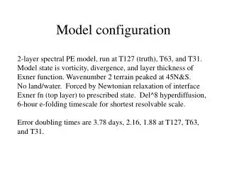
Model configuration 2-layer spectral PE model, run at T127 (truth), T63, and T31. Model state is vorticity, divergence, and layer thickness of Exner function. Wavenumber 2 terrain peaked at 45N&S. No land/water. Forced by Newtonian relaxation of interface Exner fn (top layer) to prescribed state. Del^8 hyperdiffusion, 6-hour e-folding timescale for shortest resolvable scale. Error doubling times are 3.78 days, 2.16, 1.88 at T127, T63, and T31.
Westerly upper jets in midlatitudes, more pronounced at T127, Easterly in tropics, less pronounced at T127. Subtropical easterlies at low levels.
Model Error at T31 • Model Err = M31(T [x127(t)] ) – T [x127(t+1)] where M is the forward model operator at T is the truncation operator, and superscript denotes resolution of state and/or forecast model. • x127(t+1) = M127x127(t)
Evaluating model errors in low-resolution version of high-resolution model (here in full PE model) t = 0 t =12h (compare)
Model errors show some temporal continuity, assoc’d with jet-stream dynamics.
Model errors larger at T31, but they grow faster at T63. Peaked at baroclinic scales by 2 days.
Data Assimilation Methodology • EnSRF • Additive (different flavors, next pg) or covariance inflation (uniform across domain). Additive is random sample from time series of some forecast aspect. • Cov localization with 5000 km cutoff, Gaspari/Cohn. No vertical localiz. • 208 members
8.75 J/(kg K) obs error std dev for interface height obs
Range of Experiments • 1) T127 Perfect Model (1 %) • 2) Covariance inflation (diverged) • 3) Restarted covariance inflation (10%) • 4) Perfect additive error (no infl, true samples of error) • 5) T63 additive * 1.2 • 6) T63 analogs * 1.2 • 7) T63 no bias correction * 1.2 (4, 5, and 6 bias corr’d) • 8) 24-h tendency * 0.25 • 9) climatology * 0.25 • 10) 3D-Var * 1.40 (samples of actual errs from expt 5)
Why are covariance inflation errors higher than additive error? • Model error not in subspace of forecast ensemble? (fiddled around a lot with this to come up with good explanatory graphic, to no avail).