Download
1 / 29
320 likes | 536 Views
Linkage between WRF/NMM and CMAQ. Daewon Byun (PI) C.K. Song & P. Percell University of Houston Institute for Multidimensional Air Quality Studies (IMAQS) Coauthors: Jon Pleim, Tanya Otte, Jeff Young, Rohit Mathur ASMD, Air Resources Laboratory, NOAA In partnership with U.S. EPA

E N D
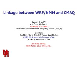
Linkage between WRF/NMM and CMAQ Daewon Byun (PI) C.K. Song & P. Percell University of Houston Institute for Multidimensional Air Quality Studies (IMAQS) Coauthors: Jon Pleim, Tanya Otte, Jeff Young, Rohit Mathur ASMD, Air Resources Laboratory, NOAA In partnership with U.S. EPA and many others… Hsin-Mu Lin, David Wong, etc…
What are the main science issues of the NWP & AQM coupling? Off-line • Consistent governing set of equations & state variables • Consistent coordinates and grid structures • Consistent numerics & physics, and parameterizations • Flexible: able to help diverse stake holders (research – regulatory application – use of different emissions inputs) • Allow studying effects of using different basic input data (e.g., Land Use/Land Cover, topography, emissions, etc) separately • Same (*) numerics & physics, and parameterizations • Same (*) coordinates and grid structures • Same (*) governing set of equations & state variables On-line * Need to check how closely the dynamics variables and trace species are matched
Components of Off-line Coupled system WRF/nmm Spatial interpolation WRF/nmm WRF/nmm Postprocessors (vertical/horizontal) WRF-CMAQ Interface Processor PREMAQ* (consistent vertical coordinate) CMAQ/E-grid CMAQ On rotated lat/long E-grid coordinate Consistent vertical coordinate Lambert conformal projection C-grid Loose coupling Tight coupling
Fully Compressible Atmosphere (OOyama, 1990) used for CMAQ Proper Coupling Requires • Follow coordinates/grid of met model • Reproduce Jacobian • Couple state variables consistently
WRF (ARW core) WRF (NMM core) WRF/NMM http://www.dtcenter.org/wrf-nmm/users/ Nonhydrostatic Mesoscale Model (NMM) core of the Weather Research and Forecasting (WRF) system was developed by NOAA/NCEP WRF/NMM + Hybrid sigma-pressure coord. + Arakawa-E + Conserves mass, momentum, enstrophy, TKE and scalar ARW (Advance Research WRF) + Terrain following hydrostatic P coord. or Terrain following sigma (ARW) + Arakawa-C + Conserves mass, momentum, dry entropy, and scalar
Define J for the Generalized Vertical Coordinate Initial Terrain-Following Hydrostatic Sigma coordinate Method 1 : sigma interface of the lower and upper layers PD: pressure of top of lower layer Method 2
Vertical Jacobian Discontinuity Problem & Solution One way to remove discontinuity For example, SIGMA LEVELS = 1.0000, .9976, .9948, .9920, .9890, .9858, .9825, .9790, .9754, .9718, .9679, .9637, .9590, .9538, .9480, .9415, .9340, .9251, .9144, .9020, .8883, .8736, .8582, .8420, .8253, .8079, .7900, .7714, .7523, .7326, .7124, .6915, .6699, .6477, .6248, .6015, .5779, .5540, .5300, .5057, .4812, .4566, .4319, .4070, .3822, .3576, .3333, .3100, .2881, .2679, .2494, .2316, .2135, .1936, .1707, .1445, .1159, .0863, .0569, .0282, .0000, Case 1) Surface pressure = 101300 Pa & sigma(kc)=0.3822, Case 2) Surface pressure = 70000 Pa & sigma(kc)=0.3822,
Horizontal E-Grid System of WRF/nmm:Rotated lat./long & Arakawa-E grid -> C-grid for CMAQ If we use diamond grid C(C,R,L,S) -> C*(CR, L,S)
(222,501) (223,501) (222,500) (223,500) dy (1,2) (2,2) dx = 0.0534521 deg. (rotated Lon.) dy = 0.0526316 deg. (rotated Lat.) (1,1) (2,1) scalar vector dx dx dx 2dx Dynamics with Semi-Staggered Arakawa E grid The E grid is essentially a superposition of two C grids. Advantages of using E-grid with dynamics solution • When only the adjustment terms in the equations of motion and continuity are considered, two large-scale solutions from each C grid may exist independently, and a noisy total solution results. • So, employ the forward-backward time differencing scheme to prevents gravity wave separation and thereby precludes the need for explicit filtering (Mesinger 1973: Mesingerand Arakawa 1976; Janji´c 1979).
Consistent coordinates and grid structures WRF/EM & CMAQ utilize Arakawa-C Grid Arakawa-B Grid (MM5) is linearly interpolated onto Arakawa-C Grid (CMAQ) Dimension for Grid Point What to do with NMM E-grid data?
How to Utilize Arakawa-E for CMAQ? • Develop a horizontal advection algorithm in CMAQ for Arakawa E-grids • Split 2-D horizontal advection operator into 1-D operators and use CMAQ-proven 1-D schemes, such as PPM, with alternation between appropriate X and Y directions • Work directly with meteorological variables on the E-grid - avoid spatial interpolation Use rotated square cells (rotated B-grid then on C-grid) Spatial distribution of dependent variables for a uniformly spaced Arakawa E-Grid E-Grid with rotated square cells. Scalar variables are considered to be constant on each grid
Advantages • Makes the E-Grid look like a B-grid whose “rows” and “columns” are along diagonal SW→NE and SE→NW lines • Can use 1-D algorithm, e.g. PPM, along these lines • CMAQ (and preprocessors) are familiar with turning B-grid data into C-grid flux point data Disadvantages • Diagonal lines of cells have variable lengths, which requires non-trivial extra book-keeping (in EGRID_MODULE.F) • Requires interpolation of wind velocities to get flux point values • Jagged boundary effect • Parallelization could be more difficult
Bookkeeping issues Grid geometry changes depending on whether the number of columns or rows is even or odd Partitioning for parallelization
Jagged Boundary Effect rotated B-grid then on C-grid Boundary values propagate into the domain because boundaries are angled 45 degree
Comparison between regular CMAQ and Option 1 Option 1: rotated B-grid then on C-grid CMAQ C-grid
Calculation Flow of WCIP/NMM Mapping Variables START get env./IOAPI variables • define grid/coord. • rotated Lat./Lon coord. • E-grid structure • calculate Dx & Dy • allocate memory xgrid and cgrid get met. data calculation for WRF/NMM - Eta1 & Eta2 - geopotential height - hydrostatic pressure - hydrometeor GRIDOUT derive dynamic fld. METCRO/DOTOUT continue END
TEST Run • Target Period : 00Z June 28 - 06Z June 30, 2006 • Horizontal Resolution : ~ 12 km
Model Configuration C-Grid E-Grid ----------------------------------------------------------------------------------------- Met. MM5 v3.6.1 WRF/NMM v2.1 (w/ Eta forecast) (w/ Eta forecast) MCIP MCIP v3.0 WCIP/NMM v1.0 BCON BCON/Standard BCON/E-grid v1.0 ICON ICON/ Standard ICON/ E-grid v1.0 CMAQ CMAQ v4.4 CMAQ/ E-grid v1.0 ----------------------------------------------------------------------------------------- + I.C. C-Grid UH-AQF/CMAQ 12km resolution output 00Z June 28, 2006 + B.C. C-Grid UH -AQF /CMAQ 36km resolution output 00Z June 28 – 06Z June 30, 2006 + Emisson None + Chem. Mech. CB-IV
Domain Configuration C-Grid E-Grid ----------------------------------------------------------------------------------------- Met. (MM5) (WRF/NMM) + nx(dx) 100(12 km) 85(0.0780 deg.*) + ny(dy) 100(12 km) 135(0.0724 deg.) + nz 43 sigma 44 hybrid sigma-P CMAQ + nx(dx) 89** 57*** + ny(dx) 89 113 + nz 23 (see COORD_23L.EXT) 23 (JP & Dis.) ----------------------------------------------------------------------------------------- * ds=sqrt(dx**2+dy**2) ~ 12 km ** As for DOT case of MCIP, nx and ny should be 90 ** As for CRO/DOT case of WCIP/NMM, nx(ny) should be 59(115)
Recommended Model Physics for WRF/NMM Microphysics: Ferrier Cumulus Convection: Betts-Miller-Janjic Shortwave Radiation: GFDL Longwave Radiation: GFDL Lateral diffusion: Smagorinsky PBL, free atmosphere: Mellor-Yamada-Janjic Surface Layer: Janjic Scheme Land-Surface: 4-layer soil model
CMAQ Results No emissions, Transport & Chemistry Only 12Z (06 CST) June 28, 2006 (12 hrs after initial time)
C-Grid E-Grid Wind PBLHCO O3 hr18
C-Grid E-Grid ZH JabobianAir temp. U-wind ---- 13000 m ---- 13000 m discontinuity
C-Grid E-Grid CO CO
C-Grid E-Grid O3 O3
Conclusion + Presented a method to cast the WRF meteorological data on CMAQ grid & coordinate structures to represent transportation of pollutants. + Developed WCIP/NMM, BCON/E-grid, ICON/E-grid, and CMAQ/E-grid + Performed simulation (WRF/NMM -> CMAQ/E-grid) was successfully done + A simple evaluation with transport and chemistry was performed Results of CMAQ/E-grid simulation is generally consist with CMAQ/C-grid but reveal properly the discrepancy of meteorological fields Future Work + To solve some unsolved problems (WRF/NMM IOAPI, etc) + More Evaluations & Documentation + Deliver the developed codes to NOAA/EPA for National AQF