Download
1 / 35
350 likes | 509 Views
Overview of combined cloud retrievals from active instruments in space. Robin Hogan University of Reading Thanks to Nicola Pounder, Julien Delanoe , Chris Westbrook, Thorwald Stein. 4 March 2014. Overview. What do we need to retrieve? Importance of classification

E N D
Overview of combined cloud retrievals from active instruments in space Robin Hogan University of Reading Thanks to Nicola Pounder, Julien Delanoe, Chris Westbrook, Thorwald Stein 4 March 2014
Overview • What do we need to retrieve? • Importance of classification • A-Train, EarthCARE and unified retrieval algorithms • General synergy retrieval framework • Sources of uncertainty • Ice retrievals • Radar plus: lidar, another radar, Doppler… which is best? • Importance of radar scattering model • Liquid cloud retrievals • The problem of drizzle • Potential exploitation of multiply scattered signal from Calipso • A mixed-phase case • Outlook This talk is limited to satellite measurements No cost functions will be shown in this talk
What do we need to retrieve? • Interaction of clouds with natural radiation depends on: • First-order importance: extinction coefficientbe • If : • Valid for SW ice & liquid, LW ice (but liquid clouds often black bodies) • Second-order importance: asymmetry factor, single-scattering albedo • Models predict or diagnose: • Liquid water content, ice water content, cloud fraction • Rain rate, snowfall rate, ice/snow/rain fall speed • Also need measures of particle size: • Effective radius is used by models: • To convert ice/liquid water content to extinction coefficient: • To parameterize asymmetry factor, single-scattering albedo • Physical size (e.g. for fall-speed calculation) • Note that ice effective radius is typically much less than physical size (~50 mm vs. ~1 mm)
Classification… • “Unified” retrieval (for EarthCARE) provides microphysical properties for all target types • Error estimates include contribution from measurement and model error • Looks impressive but is it right? Classification: Ceccaldi et al. (JGR 2013) …Retrieval Illingworth et al. (BAMS 2014)
What would EarthCARE see? • Compared to the A-Train, EarthCARE(launch 2016) has: • 7-dB more sensitive radar with Doppler capability • High spectral resolution lidar: better extinction profiles • Imager (like MODIS) and broad-band radiometer (like CERES)
General retrieval framework • One measurement one retrieved variable via empirical relationship • E.g. IWC(Z) • Two measurements two retrieved variables • Second measurement (e.g. another wavelength, Doppler) often doesn’t give independent information all the time • Top tip: make one of the retrieved variables a measure of (normalized) number concentration with good prior (e.g. temperature) • Then automatically falls back to best one-measurement retrieval • Three measurements… • Can we get a handle on other variables, e.g. ice density, particle habit? Field et al. (2005)
There are known knowns. These are things we know that we know. There are known unknowns. That is to say, there are things that we know we don't know. But there are also unknown unknowns. There are things we don't know we don't know. Donald Rumsfeld
A Rumsfeldian taxonomy • The known knowns, things we know so well no error bar is needed • Drops are spheres, density of water is 1000 kg m-3 • The known unknowns, things we can explicitly assign an well-founded error bar to in a variational retrieval • Random errors in measured quantities (e.g. photon counting errors) • Errors and error covariances in a-priori assumptions (e.g. rain number conc. parameter Nw varies climatologically with a factor of 3 spread) • The unknown unknowns where we don’t know what the error is in an assumption or model • Errors in radiative forward model, e.g. radar/lidar multiple scattering • Errors in microphysical assumptions, e.g. mass-size relationship • How do errors in classification feed through to errors in radiation? • How do we treat systematicbiases in measurements or assumptions? • (also the ignored unknowns that we are too lazy to account for!) How can we move more things into the “known unknowns” category?
Ice retrievals Radar Dual-lHogan et al. (1999) IWC(Z), IWC(Z, T) • What is the best supplement to radar reflectivity factor? DopplerMatrosov, EarthCARE CloudSat: Austin et al. (2009) Donovan et al. (2001), Okamoto et al. (2003) Delanoe and Hogan (2010), EarthCARE “unified” HSRLEarthCARE LIRAD (Platt) Chiriaco et al. (2004) MODIS etc. Radiometer CALIPSO, Klett etc. Lidar
Lidar-radar combination • Advantages • Lidar much more sensitive to thin cirrus: with radar gives great coverage • Synergy extracts lidar attenuation: exactly what we want to know • Radar-lidar ratio is very sensitive to particle size • Limitations • Signal extinguished in many deep clouds: revert to radar-only information • Tricky to use: many papers try to correct lidar for attenuation first, but it is much more accurate to use the radar to help the inversion • Retrieved lidar backscatter-to-extinction profile assumed constant with height: leads to biases if there is really a vertical gradient (problem resolved using infrared radiances or EarthCARE’s HSRL)
Additional radar information • Additional 215 GHz radar • Size info deep in cloud: complements lidar • Dependent on good radar scattering model • Doppler (e.g. EarthCARE) • Sensitive to ice density and therefore riming • Need high signal-to-noise • No use in convective clouds
Snow Simulated aggregate (Westbrook et al.) • What’s the 94 GHz backscatter cross-section of this? • Spheroid model works up to D ~ l, but not for larger particles • Rayleigh-Gans approximation works well: describe structure simply by area of particle A(z) as function of distance in direction of propagation of radiation Area of slice through particle A(z)
Radar scattering by ice 1 mm ice 1 cm snow • Hogan and Westbrook (2014) used simulated ice aggregates to derive an equation for radar backscatter: the “Self-Similar Rayleigh Gans approximation” • For snowflakes, internal structures on scale of wavelength lead to significantly higher higher backscatter than “soft spheroids” Realistic aggregate snowflake Soft spheroid
Field et al. (2005) size distributions at 0°C Circles indicate D0 of 7 mm reported from aircraft (Heymsfield et al. 2008) Lawson et al. (1998) reported D0=37 mm: 17 dB difference Impact of scattering model 4.5 dB Factor of 5 error
Ice aggregates Ice spheres Impact of ice shape on retrievals • Spheres can lead to overestimate of water content and extinction of factor of 3 • All 94-GHz radar retrievals affected in same way
Liquid cloud retrievals Radar PIA Lebsocket al. (2011) Drizzle-free: LWC(Z) CloudSat: Austin & Stephens (2001) Optically very thin: Spinhirne et al. (1989) MODIS etc. Wide-FOV Pounder et al. (2012) Radiometer Lidar
The problem with liquid clouds • 90% of liquid clouds over the oceans; 90% of those contain drizzle • Lidar signal strongly attenuated & contaminated by multiple scattering • Very useful constraints from radar path integrated attenuation (PIA) providing liquid water path (over ocean only) and MODIS providing optical depth (daytime only), but vertical profile very uncertain CloudSat radar reflectivity factor (dBZ) Where is cloud base? Calipso lidar backscatter (m-1 sr-1)
New liquid cloud retrieval • Pounder, Hogan et al. (2012) proposed variational method to retrieve extinction profile in stratocumulus exploiting the multiple scattering from multiple field-of-view lidar (use fast “multiscatter” model) • This idea works for single field-of-view lidar with footprint > 50 m • Add constraint on LWC to be no steeper than adiabatic • Calipso alone can retrieve optical depth and cloud base height • Estimated LWP can then be compared to that from CloudSat PIA • Complements other methods: land and sea, but night-time only • Forward modelled backscatter • Observed backscatter
Calipso-only retrievals (assume fixed Nd) • LWC • Effective radius • Optical depth • CloudSat PIA
A mixed-phase case Observations Unified algorithm automatically uses radar to constrain ice and lidar to constrain liquid retrievals No idea what to do with embedded liquid unseen by lidar Note that quasi-Newton scheme uses many iterations… • Retrievals
Outlook • EarthCARE is the exciting next step to the A-Train • Better ice retrievals, especially for thin ice clouds: radar 7 dB more sensitive: HSRL gives direct extinction • Doppler provides useful information on ice density and riming (as well as better retrievals of rain and drizzle rate) • On-board 3-view broadband radiometer tests for radiative consistency • What are the next steps for active cloud sensing in space? • Multiple field-of-view lidar to retrieve extinction profile in stratocu • Combined 94-215 GHz radars for particle sizing deep into ice cloud • Radar measures linear depolarization to identify and exploit multiple scattering in deep convection • Combine with Oxygen A-band spectrometer • Combine with narrow-view microwave radiometers • Better synergy algorithms with robust error estimates!
The A-Train versus EarthCARE EarthCARE (launch 2016) • ESA and JAXA • Single platform • 393-km: higher sensitivity • 94-GHz Doppler radar • 355-nm High spectral res. lidar • 3-view broad-band radiometer • Multi-spectral imager The A-Train (fully launched 2006) • NASA • Multiple platforms • 700-km orbit • CloudSat 94-GHz radar • Calipso 532/1064-nm lidar • CERES broad-band radiometer • MODIS multi-wavelength radiometer
Chilbolton 10-cm radar + UK aircraft • Reflectivity agrees well, provided Brown & Francis mass used with Dmean • Differential reflectivity agrees reasonably well for oblate spheroids CWVC IV: 21 Nov 2000
Simulated retrieval of optical depth for idealized adiabatic clouds, using spaceborne lidar with varying field of view (FOV) For FOV less than around 50 m, there is simply too little multiple scattering signal to retrieve extinction and optical depth Will this work with EarthCARE? FOV >= 55 m (e.g. Calipso) FOV <= 50 m (e.g. EarthCARE) …No!
Unified retrieval Ingredients developed Not yet completed 1. Define state variables to be retrieved (x) Use classification to specify variables describing each species at each gate Ice and snow: extinction coefficient, N0’, lidar ratio, riming factor Liquid: extinction coefficient and number concentration Rain: rain rate, drop diameter and melting ice Aerosol: number concentration, particle size and lidar ratio 2. Forward model 2a. Radar model With multiple scattering, Doppler and PIA 2b. Lidar model Including HSRL channels and multiple scattering 2c. Radiance model Solar & IR channels 4. Iteration method Derive a new state vector: quasi-Newton or Levenberg-Marquardt scheme Not converged 3. Compare to observations (y) Check for convergence Converged 5. Calculate retrieval error Error covariances & averaging kernel Proceed to next ray of data
What the results look like so far CloudSat observations CloudSat forward model Calipso observations Calipso forward model
Ice extinction coefficient Liquid water content Rain rate Aerosol extinction coefficient
Extending ice retrievals to riming snow • Retrieve a riming factor (0-1) which scales b in mass=aDb between 1.9 (Brown & Francis) and 3 (solid ice) 0.9 0.8 0.7 0.6 • Heymsfield & Westbrook (2010) fall speed vs. mass, size & area • Brown & Francis (1995) ice never falls faster than 1 m/s Brown & Francis (1995)
Examples of snow35 GHz radar at Chilbolton 1 m/s: no riming or very weak 2-3 m/s: riming? • PDF of 15-min-averaged Doppler in snow and ice (usually above a melting layer)
Assimilate also CloudSat PIA • LWC • Effective radius • Optical depth • CloudSat PIA
Retrieve number concentration • LWC • Effective radius • Optical depth • CloudSat PIA • Number concentration