Download
1 / 29
300 likes | 501 Views
Aerosol retrievals from AERONET sun/sky radiometers: Overview of - inversion principles - aerosol retrieval products - advances and perspectives.

E N D
Aerosol retrievals from AERONET sun/sky radiometers: Overview of - inversion principles - aerosol retrieval products -advances and perspectives O. Dubovik1,2, A. Sinuyk2, B.N. Holben2andAERONET team1 - University of Lille, CNRS, France2 - NASA/GSFC, Greebelt, USA The Second International Conference of Aerosol Science and Global Change August, 18-21, 2009, Hangzhou, China
AERONET Inversion Forward Model: Single Scat: ensemble of polydisperse randomly oriented spheroids (mixture of spherical and non-spherical aerosol components) Multiple Scat: (scalar) Nakajima and Tanaka, 1988, or (polarized) Lenouble et al., JQSRT, 2007 t(l), I(l,Q),P(l,Q) Optimized Numerical inversion: - Accounting for uncertainty (F11; -F12/F11 !!!) - Setting a priori constraints aerosol particle sizes, complex refractive index (SSA), Non-spherical fraction
Accounting for multiple scattering effects ASSUMPTIONS in the retrievals: • - cloud-free atmosphere; • horizontal homogeneous atmosphere; • - assumed gaseous absorption and molecular scattering; • vertically homogenous atmosphere (assumed profile of concentration !? ) • bi-directional surface reflectance assumed from MODIS observations • - accounting for polarization effects!?!
AERONET model of aerosol AERONET model of aerosol Dubovik et al., 2006 spherical: Randomly oriented spheroids : (Mishchenko et al., 1997)
Aerosol single particle scattering: ASSUMPTIONS in the retrievals: • EACH AEROSOL PARTICLE • sphere or spheroid (!!!); • homogeneous; • 1.33 ≤ n ≤ 1.6 (1.7- ???) • - 0.0005 (0 - ???) ≤ k ≤ 0.5 • n and k spectrally dependent(but smooth)
Aerosol particle size distribution Trapezoidal approximation (Twomey 1977) • ASSUMPTIONS: • dV/dlnr - volume size distribution of aerosol in total atmospheric column; • size distribution is modeled using 22 triangle size bins (0.05 ≤ R ≤ 15 m); • size distribution is smooth
Mixing of particle shapes retrieved C + (1-C) Aspect ratio distr. • ASSUMPTIONS: • - dV/dlnr - volume size distribution is the same for both components; • non-spherical - mixture of randomly oriented polydisperse spheroids; • aspect ratio distribution N(is fixed to the retrieved by Dubovik et al. 2006
Single Scattering using spheroids spheroidkernels data basefor operational modeling !!! Input:wp(Np =11), V(ri) (Ni =22 -26) K- pre-computed kernel matrices: Input: n and k • Basic Model by Mishchenko et al. 1997: • randomly oriented homogeneous spheroids • w(e) - size independent shape distribution Time: < one sec. Accuracy: < 1-3 % Range of applicability: 0.012 ≤ 2pr/l ≤ 625 (41 bins) 0.3 ≤ e ≤ 3.0 (25 bins) 1.3 ≤ n ≤ 1.7 0.0005 ≤ k ≤ 0.5 Output:t(l), w0(l), F11(Q), F12(Q),F22(Q), F33(Q),F34(Q),F44(Q)
INPUT of Forward Model AERONET retrievals are driven by 31 variables : dV/lnr - size distribution (22 values); n() and k() - ref. index (4 +4 values) Cspher(%) - spherical fraction (1 value) Complex Refractive Index at l = 0.44; 0.67; 0.87; 1.02 mm Particle Size Distribution: 0.05 mm ≤ R (22 bins) ≤ 15 mm Desert Dust Maritime Smoke
Inversion • Statistically Optimized Minimization- Fitting • (Dubovik and King, 2000) weighting Lagrange parameters • Measurements: • i=1 - optical thickness • i=2 - sky radiances • their covariances • (should depend on l and Q) • -lognormal error distributions a priori restrictions on norms of derivatives of: i=3 -size distr. variability; i=4 -n spectral variability; i=5 -k spectral variability; i=6 - limiting dV/dlnr for Rmin consistency Indicator
A priori restirctions • A priori restrictions on smoothness • (Dubovik and King, 2000) Strength of constraint Most unsmooth KNOWN size distribution norms of derivatives Meaning : m=1 -constant straight line: V(lnr)= C; m=2 -constant straight line: V(lnr)= B lnr +C; m=3 -parabola: V(lnr)= A(lnr)2 + B lnr +C;
AERONET retrieval products: - V1 - V2 - V3 • Directly retrieved parameters: • dV/dlnR - size distribution; (- dynamic errors ) • -C(t,f,c), Rv(t,f,c), (t,f,c), Reff (t,f,c) - integral parameters of dV/dlnR • n() and k () at 0.44, 0.67, 0.8, 1.02 m; (- dynamic errors ) • -Cspherical- fraction of spherical particles (- dynamic errors ) • Indirectly retrieved/estimated parameters: • popular: • - at 0.44, 0.67, 0.8, 1.02 m; (- dynamic errors ) • P11()(- dynamic errors ) and <cos()> ; • P12() and P22()- ???(- dynamic errors ) • - FTOA() and FBOA() - down ward spectral fluxes • - FTOA() andFBOA() - upward spectral fluxes • not well-known / under-developed: - S() - lidar backscattering-to-extinction ratio; (- dynamic errors ) -() - lidar depolarization ratio ; (- dynamic errors ) - FTOA and FBOA - down ward broad-band (visible) fluxes; - FTOAandFBOA- upward broad-band (visible) fluxes; - ∆FTOA and ∆FBOA - radiative forcing -∆FEffTOAand ∆FEffBOA- radiative forcing efficiency
Fine / Coarse modes parameters: Flexible separation: minimum between: 0.194 and 0.576 m 0.45mm • Integral parameters of dV/dlnR: • t - total; f - fine ; c - coarse • C(t,f,c) - Volume Concentration • Rv(t,f,c) - Mean Radius • (t,f,c) - Standard Deviation • Reff (t,f,c)- Effective Radius
Retrieval accuracy and limitations Accuracy summary Sensitivity tests by Dubovik et al. 2000 bias ∆t = ± 0.01 Effective wide angular coverage t(0.44) ≤ 0.2 0.05 80-100% 0.05-0.07 t(0.44) ≥ 0.5 0.025 50% 0.03 Real Part Imaginary Part SSA Size Distribution: Nonsphericity biases Random errors
Error estimates: Important Error Factors: - Aerosol Loading - Scattering Angle Range - Number of Angles (homogeneity) - Number of spectral channels - Aerosol Type etc. New strategy: Errors are to be provided in each single retrievals for all retrieved parameters
Dubovik 2004 Rigorous ERRORS estimates:General case: large number of unknowns and redundant measurements U - matrix of partial derivatives in the vicinity of solution Above is valid: - in linear approximation - for Normal Noise - strongly dependent on a priori constraints - very challenging in most interesting cases
Size distribution Input ERRORS and biases Random (normally distributed with 0 means): - optical thickness: s = 0.015 COS(SZA) - sky-radiances: ssky = 3% - a priori: ssky/ i 100 - 300 % (Dubovik and King, 2000) Biases (constant): - optical thickness: 0.015 COS(SZA) - sky-radiances: 3% + obtained misfit - a priori: 100 - 300 % The error estimates are calculated twice with + and - bias.
Examples of error estimates high loading low loading
Dubovik 2004 ERRORS estimates for thefunctions of the retrieved parameters:0, Pii(), etc. - vector of partial derivatives in the vicinity of solution Above is valid: - in linear approximation - for Normal Noise - strongly dependent on a priori constraints
Statistical variability of SSA errors A. Sinyuk The Second International Conference of Aerosol Science and Global Change August, 18-21, 2009, Hangzhou, China
Statistical variability of errors for sphericity parameter A. Sinyuk The Second International Conference of Aerosol Science and Global Change August, 18-21, 2009, Hangzhou, China
Lidar Ratio CALIOP Data: Lidars are sensitive to: Extinction S=19 S=50
Optics Microphysics Volten et al. Volten et al. 2001
Lidar Ratio from AERONET climatology Cattrall et al., 2005
Size Dependence of Depolarization for Randomly Oriented Spheroids Log-normal monomodal dV(r)/dlnr : sv = 0.5, l = 0.44 mm, n = 1.4, k = 0.005 F22(Q)/ F11(Q) Lidar signal depolarization F22/ F11
AERONET estimated broad-band fluxes in solar spectrum FTOA and FBOA FTOA and FBOA • Integrations details: • min = 0.2m, max = 4.0 m; • more than 200 points of integration between; Aerosol: • dV/dlnR - retrieved • n() and k() are interpolated/extrapolated; • from n(i) and k(i) retrieved; • Radiative transfer code uses 12 moments for P11() • Surface: • Surface reflection is Lambertian; • Values of surface refelctance are interpolated/ extrapolated from MODIS data values Gases: • Gaseous absorption is calculated using correlated k-distributions implemented by P. Dubuisson Validation studies: Derimian et al. 2008 Garcia et al. 2008 ( FBOA ~ 10% agreement ) Size distribution
Aerosol AERONET estimated aerosol forcing in solar spectrum size Radiative forcing: ∆FTOA = F0TOA - FTOA ∆FBOA = F0BOA - FBOA Radiative forcing efficiency: ∆FEffTOA = ∆FTOA/0.55 ∆FEffBOA = ∆FBOA/0.55 Sol. Radiance,mWcm-2str-1mm-1 Terr. Radiance,mWcm-2str-1mm-1 • Finding by Derimian et al. 2008: • importance of non-sphericity: up to 10% overestimation of ∆FTOA/BOA; Suggested improvementsby Derimian and others: • Use net fluxes: ∆FBOA = (F0BOA-F0BOA) - (FBOA-FBOA) • Estimate daily forcing • Estimates of IR fluxes/forcing Size distribution
Shuster, et al. 2005, 2009 ? n() k() Water+ Soluble+ Insoluble+ +BC m()= m( a1 m1(); a2 m2(); a3 m3())
Improving retrieval products: - releasing dynamic errors; - polishing Flux and Forcing products (ref: Y. Derimian talk) - providing lidar ratios; - providing depolarizations ratios; 2. Updating scattering model: - including surface roughness for spheroids - expanding ranges of n and k 3. New Inversion developments: - inversion of polarized data (ref: Z. Li talk) - AERONET/MODIS/PARASOL (ref: A. Sinuyk talk) - AERONET/CALIPSO (ref: A. Sinuyk work ) - inversion of daily data, combining with PARASOL (ref: O. Dubovik talk ) - deriving composition information (ref: G. Shuster work) Perspectives: The Second International Conference of Aerosol Science and Global Change August, 18-21, 2009, Hangzhou, China