Download
1 / 19
200 likes | 411 Views
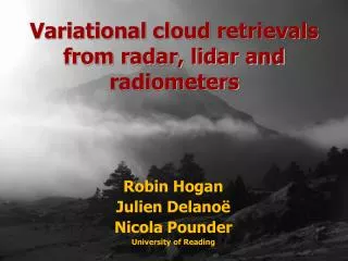
Robin Hogan Julien Delano ë Nicola Pounder University of Reading. Variational cloud retrievals from radar, lidar and radiometers. Introduction. Best estimate of the atmospheric state from instrument synergy Use a variational framework / optimal estimation theory

E N D
Robin Hogan JulienDelanoë Nicola Pounder University of Reading Variational cloud retrievals from radar, lidar and radiometers
Introduction • Best estimate of the atmospheric state from instrument synergy • Use a variational framework / optimal estimation theory • Some important measurements are integral constraints • E.g. microwave, infrared and visible radiances • Affected by all cloud types in profile, plus aerosol and precipitation • Hence need to retrieve different particle types simultaneously • Funded by ESA and NERC to develop unified retrieval algorithm • For application to EarthCARE • Will be tested on ground-based, airborne and A-train data • Algorithm components • Target classification input • State variables • Minimization techniques: Gauss-Newton vs. Gradient-Descent • Status of forward models and their adjoints • Progress with individual target types • Ice clouds • Liquid clouds
1. New ray of data: define state vector Use classification to specify variables describing each species at each gate Ice: extinction coefficient , N0’, lidar extinction-to-backscatter ratio Liquid: extinction coefficient and number concentration Rain: rain rate and mean drop diameter Aerosol: extinction coefficient, particle size and lidar ratio 6. Iteration method Derive a new state vector Either Gauss-Newton or quasi-Newton scheme Retrieval framework 2. Convert state vector to radar-lidar resolution Often the state vector will contain a low resolution description of the profile 3. Forward model 3a. Radar model Including surface return and multiple scattering 3c. Radiance model Solar and IR channels 3b. Lidar model Including HSRL channels and multiple scattering Ingredients developed before In progress Not yet developed Not converged 4. Compare to observations Check for convergence 5. Convert Jacobian/adjoint to state-vector resolution Initially will be at the radar-lidar resolution Converged 7. Calculate retrieval error Error covariances and averaging kernel Proceed to next ray of data
Target classification • In Cloudnet we used radar and lidar to provide a detailed discrimination of target types (Illingworth et al. 2007): • A similar approach has been used by Julien Delanoe on CloudSat and Calipso using the one-instrument products as a starting point: • More detailed classifications could distinguish “warm” and “cold” rain (implying different size distributions) and different aerosol types
Example from the AMF in Niamey 94-GHz radar reflectivity Forward model at final iteration 532-nm lidar backscatter 94-GHz radar reflectivity Observations 532-nm lidar backscatter
Results: radar+lidar only Large error where only one instrument detects the cloud Retrievals in regions where radar or lidar detects the cloud Retrieved visible extinction coefficient Retrieved effective radius Retrieval error in ln(extinction)
Results: radar, lidar, SEVERI radiances Cloud-top error greatly reduced Retrieval error in ln(extinction) TOA radiances increase retrieved optical depth and decrease particle size near cloud top Delanoe & Hogan (JGR 2008) Retrieved visible extinction coefficient Retrieved effective radius
Proposed list of retrieved variables held in the state vector x Unified algorithm: state variables Ice clouds follows Delanoe & Hogan (2008); Snow & riming in convective clouds needs to be added Liquid clouds currently being tackled Basic rain to be added shortly; Full representation later Basic aerosols to be added shortly; Full representation via collaboration?
The cost function Some elements of x are constrained by an a priori estimate The forward model H(x) predicts the observations from the state vector x Each observation yi is weighted by the inverse of its error variance This term penalizes curvature in the extinction profile • The essence of the method is to find the state vector x that minimizes a cost function: + Smoothness constraints
Gauss-Newton method See Rodgers’ book (p85): write the cost function in matrix form: Define its gradient (a vector): …and its second derivative (a matrix): Approximate J as quadratic and apply this: Advantage: rapid convergence (instant convergence for linear problems) Another advantage: get the error covariance of the solution “for free” Disadvantage: need the Jacobian matrix of every forward model: can be expensive for larger problems
Gradient descent methods Just use gradient information: Advantage: we don’t need to calculate the Jacobian so forward model is cheaper! Disadvantage: more iterations needed since we don’t know curvature of J(x) Use a quasi-Newton method to get the search direction, such as BFGS used by ECMWF: builds up an approximate form of the second derivative to get improved convergence Scales well for large x Disadvantage: poorer estimate of the error at the end Why don’t we need the Jacobian H? The “adjoint” of a forward model takes as input the vector {.} and outputs the vector Jobs without needing to calculate the matrix H on the way Adjoint can be coded to be only ~3 times slower than original forward model Tricky coding for newcomers, although some automatic code generators exist Typical convergence behaviour
Forward model components • From state vector x to forward modelled observations H(x)... Jacobian matrix H=y/x x Ice & snow Liquid cloud Rain Aerosol Lookup tables to obtain profiles of extinction, scattering & backscatter coefficients, asymmetry factor Ice/radar Ice/lidar Ice/radiometer Liquid/radar Liquid/lidar Liquid/radiometer Computationally expensive matrix-matrix multiplications: the most expensive part of the entire algorithm Rain/radar Rain/lidar Rain/radiometer Aerosol/radiometer Aerosol/lidar Sum the contributions from each constituent Lidar scattering profile Radar scattering profile Radiometer scattering profile Radiative transfer models Gradient of radar measurements with respect to radar inputs Gradient of lidar measurements with respect to lidar inputs Gradient of radiometer measurements with respect to radiometer inputs H(x) Lidar forward modelled obs Radar forward modelled obs Radiometer forward modelled obs Jacobian part of radiative transfer models
Equivalent adjoint method • From state vector x to forward modelled observations H(x)... Gradient of cost function (vector) J/x=HTy* x Ice & snow Liquid cloud Rain Aerosol Lookup tables to obtain profiles of extinction, scattering & backscatter coefficients, asymmetry factor Ice/radar Ice/lidar Ice/radiometer Liquid/radar Liquid/lidar Liquid/radiometer Vector-matrix multiplications: around the same cost as the original forward operations Rain/radar Rain/lidar Rain/radiometer Aerosol/radiometer Aerosol/lidar Sum the contributions from each constituent Lidar scattering profile Radar scattering profile Radiometer scattering profile Radiative transfer models Adjoint of radar model (vector) Adjoint of lidar model (vector) Adjoint of radiometer model H(x) Lidar forward modelled obs Radar forward modelled obs Radiometer forward modelled obs Adjoint of radiative transfer models
First part of a forward model is the scattering and fall-speed model Same methods typically used for all radiometer and lidar channels Radar and Doppler model uses another set of methods Graupel and melting ice still uncertain; but normal ice is decided... Scattering models
Computational cost can scale with number of points describing vertical profile N; we can cope with an N2dependencebut not N3 Radiative transfer forward models • Lidar uses PVC+TDTS (N2), radar uses single-scattering+TDTS (N2) • Jacobian of TDTS is too expensive: N3 • We have recently coded adjoint of multiple scattering models • Future work: depolarization forward model with multiple scattering • Infrared will probably use RTTOV, solar radiances will use LIDORT • Both currently being tested by Julien Delanoe
Gradient constraint • We have a good constraint on the gradient of the state variables with height for: • LWC in stratocu (adiabatic profile, particularly near cloud base) • Rain rate (fast falling so little variation with height expected) • Not suitable for the usual “a priori” constraint • Solution: add an extra term to the cost function to penalize deviations from gradient c: A. Slingo, S. Nichols and J. Schmetz, Q. J. R. Met. Soc. 1982
Example in liquid clouds • Using simulated observations: • Triangular cloud observed by a 1- or 2-field-of-view lidar • Retrieval uses Levenberg-Marquardt minimization with Hogan and Battaglia (2008) model for lidar multiple scattering Two FOVs: very good performance One 10-m footprint: saturates at optical depth=5 One 100-m footprint: multiple scattering helps! One 10-m footprint with gradient constraint: can extrapolate downwards successfully Optical depth=30 Footprint=100m Footprint=600m
Progress • Done: • C++: object orientation allows code to be completely flexible: observations can be added and removed without needing to keep track of indices to matrices, so same code can be applied to different observing systems • Code to generate particle scattering libraries in NetCDF files • Adjoint of radar and lidar forward models with multiple scattering and HSRL/Raman support • Radar/lidar model interfaced and cost function can be calculated • In progress / future work: • Interface to BFGS algorithm (e.g. in GNU Scientific Library) • Implement ice, liquid, aerosol and rain constituents • Interface to radiance models • Test on a range of ground-based and spaceborne instruments • Test using ECSIM observational simulator • Apply to large datasets of ground-based observations…