Download
1 / 21
220 likes | 280 Views
Explore different types of variables, levels of measurement (nominal, ordinal, interval, ratio), and data set creation. Learn about univariate, bivariate, and multivariate analyses, the purpose of descriptive and inferential analysis, and how to choose between parametric and non-parametric tests. Discover frequency distributions, graphical representations, measures of central tendency, and variability. Gain insights into errors, selecting statistical tests based on sample size and variable measurement levels, and more.

E N D
Introduction to Quantitative Research Analysis and SPSS SW242 – Session 6 Slides
Creation & Description of a Data Set • Four Levels of Measurement • Nominal, ordinal, interval, ratio • Variable Types • Independent Variables (IV), Dependent Variables (DV) • Moderator variables • Discrete Variables • Finite answers, limited by measurement e.g. test scores, • Continuous variables • All values possible (GPA not exceed 5.0) • Dichotomous variable • Only 2 values, yes or no, male or female • Binary variable • Assign a0 (yes) or1 (no) to indicate presence or absence of something
Categories of Analysis Number of Variables Analyzed Univariate analyses • Examine the distribution of value categories (nominal/ordinal) or values (interval or ratio) Bivariate analyses • Examine the relationship between two variables Multivariate analyses • Simultaneously examine the relationship among three or more variables
Purpose of Analysis Descriptive • Summaries of population studied (parameters) • Preliminary to further analysis Inferential • Used with sample from total population and how well can results be generalized to total population
Parametric vs. Non-Parametric Parametric Tests require: • One variable (usually the DV) is at the interval or ratio level of measurement • DV is normally distributed in the population; independent samples should have equal or near equal variances • Cases selected independently (random selection or random assignment) • Robustness how many and which assumptions above can be violated without affecting the result (delineated in advanced texts).
Parametric vs. Non-Parametric Nonparametric Tests involve nominal or ordinal level data when: • Samples complied form different populations and we want to compare the distribution of a single variable within each of them • Variables are nominal or can only be rank ordered • Very small samples: e.g. only 6 or 7 are available • Statistical power is low, increases with sample size (as with parametric tests)
Creation & Description of a Data Set Frequency Distributions: • An array is an arrangement of data from smallest to highest • Absolute/simple frequency distribution displays number of times a value occurs (all levels of measurement) • Cumulative frequency distribution adds cases together so that it last number in distribution is the total number of cases observed • Percentage distribution adds the percent of occurrence in the table • Cumulative Percentage
Graphical Representations • Bar Graph/Histogram (bars touch) • Line Graph/Frequency Polygon • Pie Chart • Keep graphs simple. • Limit to salient information info. • Collapse categories/distributions when possible.
Measures of Central Tendency Typical representation of data, e.g. find a number or groups of numbers that is most representative of a dataset. The three types include: • Mode • Values within a dataset that occur most frequently, if two occur equally then bimodal distribution, etc. • Median • The value in the exact middle of a linear array, mean between 2 values if even number of values. • Mean: arithmetic mean • Trimmed mean (outliers removed) minimize effect of extreme outliers • Weighted mean: compute an average for values that are not equally weighted (proportionate / disproportionate sampling)
Measures of Central Tendency • Variability/Dispersion • Nominal or Ordinal use a frequency distribution or graph (bar chart) • Interval or ratio use range • Range = maximum value – minimum value +1 • Informs about the number of values that exist between the ends of the distribution e.g. 31 to 46 --there are potentially 16 values possible. The larger the range, the greater the variability. However, outliers make the range misleading. Therefore use median, or mean and standard deviation whenever possible for interval & ratio data.
Errors (continued) • The smaller the p value, the less likelihood of committing a type I, the greater the p value, the greater the chance of a type II error. p values range from 0 (total significance) to 1.0 (least significance). • Generally p values less than .05 are considered significant, while those more than .05 are not.
How to Select a Statistical Test • Sampling Method Used • How was the sample selected? • What is the size of the sample? • Were the samples related? • Was probability sampling used? • What type of variables were used • Variable Distribution among Population • Evenly distributed? • Judgment call
How to Select a Statistical Test • Level of Measurement of the Independent & Dependent Variables • Inclusionary/ exclusionary criteria (screening mechanisms) • Variable measurement levels (nominal, ordinal, etc.) • Measurement precision (best measurement level used). Use of low level measurement reduces the availability of stronger statistical techniques.
How to Select a Statistical Test Statistical Power (Reduction in Type II error) • True relationship between variables is strong not weak • Variability of variables is small rather than large • A higher p value is used (e.g. .1 vs .05) thereby increases risk of Type I error • Directional hypothesis used (one tailed) • Large sample versus a small sample (power analysis) • Cost effective sample just right for analysis • Avoid too small a sample since even if the IV is effective, it would not yield a statistically significant relationship
Introduction to SPSS • Originally it was an acronym of Statistical Package for the Social Science but now it stands for Statistical Product and Service Solutions • SPSS is one of the most popular statistical packages which can perform highly complex data manipulation and analysis with simple instructions
How to Open SPSS • Go to START • Click on PROGRAMS • Click on SPSS INC • Click on SPSS 19 or 20
Basic Structure of SPSS There are two different windows in SPSS • 1st – Data Editor Window - shows data in two forms • Data view • Variable view • 2nd – Output viewer Window – shows results of data analysis
Data View vs. Variable View • Data view • Rows are cases • Columns are variables • Variable view • Rows define the variables • Name, Type, Width, Decimals, Label, Missing, etc. • Scale – age, weight, income • Nominal – categories that cannot be ranked (ID number) • Ordinal – categories that can be ranked (level of satisfaction)
Videos about Statistics and SPSS The Basics: Descriptive and Inferential Statistics – 2.51 minutes: http://www.youtube.com/watch?v=oHGr0M3TIcA SPSS Video Tutor – 11.20 minutes: http://blip.tv/spssvideotutor/spss-video-tutorial-introduction-to-spss-4014884 Intro to SPSS – 9.57 minutes: http://www.youtube.com/watch?v=eTHvlEzS7qQ