Introduction to Quantitative Data Analysis
Introduction to Quantitative Data Analysis. Quantitative Data Analysis. Types of Statistics Descriptive Inferential—probabilistic sampling techniques, notion of random Data Preparation (Coding & Cleaning Data) Common Ways of Presenting Statistics Tables Charts Graphs.


Introduction to Quantitative Data Analysis
E N D
Presentation Transcript
Quantitative Data Analysis • Types of Statistics • Descriptive • Inferential—probabilistic sampling techniques, notion of random • Data Preparation (Coding & Cleaning Data) • Common Ways of Presenting Statistics • Tables • Charts • Graphs
Presenting Data (Raw Data) Regan, T. (1985). In search of sobriety: Identifying factors contributing to the recovery from alcoholism. Kentville, NS.
univariate:= one variable “raw count” (frequencies, percentages) Simple Univariate Tables of Frequency Distributions and Percentages Neuman (2000: 318)
Example: Raw Data Frequencies Revision of Example: Collapsing Categories and Treatment of Missing Data in Tables Johnson, A. G. (1977). Social Statistics Without Tears. Toronto: McGraw Hill.
Types of Missing Data • Examples: Non-response, don’t know, refusal etc. • Categories of missing data • Missing data completely at random (MCAR) • Equipment malfunction, illness etc… • Missing data at random • Can be explained by controlling for another variable • Missing data that is not random
Some techniques for dealing with missing data • Omission (may involve using statistical techniques or logie to decide who to omit, ex. Add all like cases based on other responses) • Imputation (guess at what the likely responses would be by comparing with other response patterns) • Match other characteristics • Distribute by equally or use weighted responses
Comparison of % distributions and without non respondents Treatment of Missing Data (Ommison vs. Inclusion) Table 5-1 Alienation of Workers Level of Alienation F % High 30 14 Medium 100 48 Low 20 10 No Response 60 29 (Total) 210 100 Table 5-1 Alienation of Workers Level of Alienation F % High 30 20 Medium 100 67 Low 20 13 (Total) 150 100
Comparison with high & medium alienation collapsed Treatment of Missing Data & collapsing categories (creating new variables after data collection) Table 5-1 Alienation of Workers Level of Alienation F % High & Medium 130 62 Low 20 10 No Response 60 29 (Total) 210 100 Table 5-1 Alienation of Workers Level of Alienation F % High & Medium 130 87 Low 20 13 (Total) 150 100 Non-respondents eliminated Non-respondents included
Comparison with medium & low collapsed Treatment of Missing Data Table 5-1 Alienation of Workers Level of Alienation F % High 30 14 Medium & Low 120 58 No Response 60 29 (Total) 210 100 Table 5-1 Alienation of Workers Level of Alienation F % High 30 20 Medium & Low 120 80 (Total) 150 100 Non-respondents eliminated Non-respondents included
Comparison of two different ways of collapsing response categories Effects of Collapsing Response Categories Table 5-1 Alienation of Workers Level of Alienation F % High & Medium 130 87 Low 20 13 (Total) 150 100 Table 5-1 Alienation of Workers Level of Alienation F % High 30 20 Medium & Low 120 80 (Total) 150 100
Collapsing categories (U.N. example) Babbie, E. (1995). The practice of social research Belmont, CA: Wadsworth
Collapsing Categories & omitting missing data Babbie, E. (1995). The practice of social research Belmont, CA: Wadsworth
Grouping Response Categories • To make new categories • Facilitate analysis of trends • But decisions have effects on the interpretation of patterns • Importance of understanding logic, conceptual and operational definitions • Same data can produce totally different-looking results
Bivariate Tables (Cross Tabulations): Tables Presenting Relationship between Two Variables Singleton, R., Straits, B. & Straits, M. (1993) Approaches to social research. Toronto: Oxford
Expected outcomes (Null Hypothesis) Singleton, R., Straits, B. & Straits, M. (1993) Approaches to social research. Toronto: Oxford
Interpretation issues (Bivariate Tables) • Percentages within categories of attributes of independent variable • In example: • Independent variable: gender • Dependent variable: fear of walking alone at night • Women more afraid than men
Styles of Presentation of Percentaged Tables (Bivariate) • Table 1. Percentage in support of strike by type of school • Percent supporting • Type of School Strike • Secondary 60% • (800) • Elementary 30% • (1000) • __________________________________________________________ • = .30 N = 1800 Dependent Variable Independent Variable Serial Number Descriptive Caption Variable One category of dichotomous dependent variable Categories Marginals for independent variable Total Sample Percentage difference (epsilon)
Factors to consider when reading table • Sampling technique? Or total population? • Conceptual & operational definitions (Validity & reliability issues) • What measure was used? • How was it used? • Data preparation and cleaning issues (treatment of inconsistencies, non-responses etc..) • Data Analysis issues
Other Ways of Presenting Same Data & Interpretation Issues • Deciding on Direction of Calculation of Percentages? • Depends on Objectives (Research Questions), for example: • Are we interested in the patterns within each school type? • Are we interested in overall support of strike?
Other Ways of Presenting Bivariate Relationships in tabular form (ex. Ratios)
In, Say it with Figures, Hans Zeisel presents the following data: Control variables: Trivariate Tables Men/Women Drivers Automobile Accidents by Sex and Distance Driven ---------------------------------------------------------------------------- Distance Under 10,000 kmOver 10,000 km Per Cent Per Cent Accident Free Accident Free Women 75% 48% (5,035) (1,915) Men 75% 48% (2,070) (5,010) ---------------------------------------------------------------------------- Automobile Accidents by Sex ------------------------------------------ Per Cent Accident Free Women 68% (6,950) Men 56% (7,080) ------------------------------------------ Women have fewer accidents than men because women tend to drive less frequently than do men, and people who drive less frequently tend to have fewer accidents
Another Way to Present Percentaged Tables (Trivariate) Dependent Variable Independent Variable • Table 2. Percentage who support strike by type of school and sex • Sex • Female Per cent Male Per cent • Type of Schoolsupporting strikesupporting strike • Secondary 60% 60% • (400) (400) • Elementary 30% 30% • (900) (100) • __________________________________________________________ Female = .30 : Male = .30 N = 1800 Control variable Categories of control variable Control variable
Common Types of Charts & Graphs • Bar charts • Histograms • Pie Charts • Line Graphs/Polygons • Scattergrams
Bar Chart • Parallel bars or rectangles with lengths proportional to the frequency with which specified quantities occur in a set of data • graphic representation of frequency distribution, • generally used for discrete data.
Bar Chart with break • World Population Growth Showing Projections (Time to add billions) Click for source
Histograms • graphically representing grouped data of a frequency distribution • baseline typically depicts the classes, and the vertical scale represents the frequencies or percentages • for continuous data. Example • In a survey of people between the age of 18 and 74 to determine the number of bike users categorized by age groups. • Q. Which age-group do you belong to?18 to 2425 to 3435 to 4445 to 5455 to 6465 to 74
Pie Chart Example: 2004 Election Results of EU • circular chart • divided into sectors, illustrating relative magnitudes or frequencies. • arc length of each sector (and consequently its centralangle and area), is proportional to the quantity it represents. • sectors create a full disk. (link to source & data)
exploded pie chart Example: 2004 Election Results of EU • one or more sectors separated from the rest of the disk
Presentation of identical data in pie and bar charts Problem with pie charts: easier to compare bar charts visually & to see differences in proportions
Line and Scatter Charts (Graph) • starts with mapping quantitative data points. • usually a dot or a small circle represents a single data point. • one mark (point) for every data point • visual distribution of the data • When both variables are quantitative, the line segment that connects the two points on the chart expresses a slope • Slope can be visually interpreted relative to the slope of other lines.
Frequency Polygon Showing Same Data (Graph Plotting Frequency Distribution)
Common types of Distributions • Normal Distribution (bell-shaped curve) • Skewed Distributions • Bi-Modal Distributions
Normal Distribution Neuman (2000: 319)
Skewed Distributions Neuman (2000: 319)
Combining Quantitative & Qualitative Info. In Graphs: Temperatures during Napoleon’s March (E. Tufte)
Example of Bad choice of graphic representation Data discrete Connecting dots does not make sense because Measures of colours are nominal here Line Chart (Poor example)
Same data presented using different scales for x and y axis Design & Interpretation Issues: Choice of Scales
Core Notions in Basic Univariate Statistics • Ways of describing data about one variable (“uni”=one) • Measures of central tendency • Summarize information about one variable (“averages”) • Measures of dispersion • Variations or “spread”
Measures of Central Tendency • summarize information about one variable in single number • Mode • Median • Mean • Use of Measures of Central Tendency • to summarize common “overall” “centralized” trends • doesn’t show variability, spread, dispersion
most common or frequently occurring case (for all types of data) Mode Babbie (1995: 378)
middle point (only for ordinal, interval or ratio data) Median Babbie (1995: 378)
“average” = sum of values divided by number of cases (only for ratio and interval data) Mean (arithmetic mean) Babbie (1995: 378)
Normal Distribution & Measures of Central Tendency Neuman (2000: 319)