Introduction to SPSS
3.47k likes | 6.93k Views
Introduction to SPSS. Data types and SPSS data entry and analysis. In this session. What does SPSS look like? Types of data (revision) Data Entry in SPSS Simple charts in SPSS Summary statistics Contingency tables and crosstabulations Scatterplots and correlations

Introduction to SPSS
E N D
Presentation Transcript
Introduction to SPSS Data types and SPSS data entry and analysis
In this session • What does SPSS look like? • Types of data (revision) • Data Entry in SPSS • Simple charts in SPSS • Summary statistics • Contingency tables and crosstabulations • Scatterplots and correlations • Tests of differences of means
Aspects of SPSS • Menus - Analyse and Charts esp. • Spreadsheet view of data • Rows are cases (people, respondents etc.) • Columns are Variables • Variable view of data • Shows detail of each variable type
In SPSS • We change ticks etc. on a questionnaire into numbers • One number for each variable for each case • How we do this depends on the type of variable/data
Types of data • Nominal • Ranked • Scales/measures • Mixed types • Text answers (open ended questions)
Nominal (categorical) • order is arbitrary • e.g. sex, country of birth, personality type, yes or no. • Use numeric in SPSS and give value labels. (e.g. 1=Female, 2=Male, 99=Missing) (e.g. 1=Yes, 2=No, 99=Missing) (e.g. 1=UK, 2=Ireland, 3=Pakistan, 4=India, 5=other, 99=Missing)
Ranks or Ordinal • in order, 1st, 2nd, 3rd etc. • e.g. status, social class • Use numeric in SPSS with value labels • E.g. 1=Working class, 2=Middle class, 3=Upper class • E.g. Class of degree, 1=First, 2=Upper second, 3=Lower second, 4=Third, 5=Ordinary, 99=Missing
Measures, scales • Interval - equal units • e.g. IQ • Ratio - equal units, zero on scale • e.g. height, income, family size, age • Makes sense to say one value is twice another • Use numeric (or comma, dot or scientific) in SPSS • E.g. family size, 1, 2, 3, 4 etc. • E.g. income per year, 25000, 14500, 18650 etc.
Mixed type • Categorised data • Actually ranked, but used to identify categories or groups • e.g. age groups • = ratio data put into groups • Use numeric in SPSS and use value labels. • E.g. Age group, 1=‘Under 18’, 2=‘18-24’, 3=‘25-34’, 4=‘35-44’, 5=‘45-54’, 6=‘55 or greater’
Text answers • E.g. answers to open-ended questions • Either enter text as given (Use String in SPSS) • Or • Code or classify answers into one of a small number types. (Use numeric/nominal in SPSS)
Data Entry in SPSS • Video by Andy Field
Frequency counts • Used with categorical and ranked variables • e.g. gender of students taking Health and Illness option
e.g. Number of GCSEs passed by students taking Health and Illness option
Central Tendency • Mean • = average value • sum of all the values divided by the number of values • Mode • = the most frequent value in a distribution • (N.B. it is possible to have 2 or more modes, e.g. bimodal distribution) • Median • = the half-way value, or the value that divides the ordered distribution in the middle • The middle score when scores are ordered • N.B. need to put values into order first
Dispersion and variability • Quartiles • The three values that split the sorted data into four equal parts. • Second Quartile = median. • Lower quartile = median of lower half of the data • Upper quartile = median of upper half of the data • Need to order the individuals first • One quarter of the individuals are in each inter-quartile range
Used on Box Plot Age of Health and Illness students Upper quartile Median Lower quartile
Variance • Average deviation from the mean, squared • 5.20 is the Sum of Squares • This depends on number of individuals so we divide by n (5) • Gives 1.04 which is the variance
Standard Deviation • The variance has one problem: it is measured in units squared. • This isn’t a very meaningful metric so we take the square root value. • This is the Standard Deviation
Using SPSS • ‘Analyse>Descriptive>Explore’ menu. • Gives mean, median, SD, variance, min, max, range, skew and kurtosis. • Can also produce stem and leaf, and histogram.
Charts in SPSS • Use ‘Chart Builder’ from ‘Graph’ menu or the Legacy menu • And/or double click chart to edit it. • E.g. double click to edit bars (e.g. to change from colour to fill pattern). • Do this in SPSS first before cut and paste to Word • Label the chart (in SPSS or in Word)
Stem and leaf plots • e.g. age of students taking Health and Illness option • good at showing • distribution of data • outliers • range
Box Plot Fill colour changed. N.B. numbers refer to case numbers.
Histograms and bar charts • Length/height of bar indicates frequency
Histogram Fill pattern suitable for black and white printing
Changing the bin size Bin size made smaller to show more bars
Pie chart • angle of segment indicates proportion of the whole
Pie Chart Shadow and one slice moved out for emphasis
Analysing relationships • Contingency tables or crosstabulations • Compares nominal/categorical variables • But can include ordinal variables • N.B. table contains counts (= frequency data) • One variable on horizontal axis • One variable on vertical axis • Row and column total counts known as marginals
Example • In the Health and Illness class, are women more likely to be under 21 than men?
Crosstabulations • e.g. • Use column and row percentages to look for relationships
Chi-square ² Cross tabulations and Chi-square are tests that can be used to look for a relationship between two variables: • When the variables are categorical so the data are nominal (or frequency). • For example, if we wanted to look at the relationship between gender and age. • There are several different types of Chi-square (²), we will be using the 2 x 2 Chi-square
Another example • The Bank employees data
Chi-Square analysis on SPSS • http://www.youtube.com/watch?v=Ahs8jS5mJKk4m15s • http://www.youtube.com/watch?v=IRCzOD27NQU • From 6m:30s to 9m:50s • http://www.youtube.com/watch?v=532QXt1PM-Q&feature=plcp&context=C3ba91a4UDOEgsToPDskJ-ABupdp-Yfvuf4j4fJGzV12m30s
Low values in cells • Get SPSS to output expected values • Look where these are <5 • Consider recoding to combine cols or rows
Tabulating questionnaire responses • Categorical survey data often “collapsed” for purposes of data analysis An analysis on a sample of 2 (e.g. Black African) would not have been very meaningful!
Recoding variables • http://www.youtube.com/watch?v=uzQ_522F2SM&feature=related • Ignore t-test for now 6m11s • http://www.youtube.com/watch?v=FUoYZ_f6Lxc • Uses old version of SPSS, no submenu now. 6m
Scatterplots and correlations • Looks for association between variables, e.g. • Population size and GDP • crime and unemployment rates • height and weight • Both variables must be rank, interval or ratio (scale or ordinal in SPSS). • Thus cannot use variables like, gender, ethnicity, town of birth, occupation.
Scatterplots • e.g. age (in years) versus Number of GCSEs
Interpretation • As Y increases X increases • Called correlation • Regression line model in red
Correlation measures association not causation • The older the child the better s/he is at reading • The less your income the greater the risk of schizophrenia • Height correlates with weight • But weight does not cause height • Height is one of the causes of weight (also body shape, diet, fitness level etc.) • Numbers of ice creams sold is correlated with the rate of drowning • Ice creams do not cause drowning (nor vice versa) • Third variable involved – people swim more and buy more ice creams when it’s warm
Scatterplot in SPSS • Use Graph menu • http://www.youtube.com/watch?v=74BjgPQvIEg8m34s • http://www.youtube.com/watch?v=blfflA-34pQ&feature=related4m04s • http://www.youtube.com/watch?v=UVylQoG4hZM1m50s, ignore polynomial regression
Modifying the Scatterplot • http://www.youtube.com/watch?v=803YCYA2AoQ&feature=related4m04s • http://www.youtube.com/watch?v=vPzvuMuVXk8&feature=related3m40s
If mixed data sets • Change point icon and/or colour to see different subsets. • Overall data may have no relationship but subsets might. • E.g. show male and female respondents. • Use Chart builder