Download
1 / 31
320 likes | 550 Views
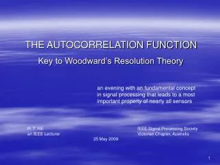
an evening with an fundamental concept in signal processing that leads to a most important property of nearly all sensors. R. T. Hill IEEE Signal Processing Society an IEEE Lecturer Victorian Chapter, Australia 25 May 2009.

E N D
an evening with an fundamental concept in signal processing that leads to a most important property of nearly all sensors R. T. Hill IEEE Signal Processing Society an IEEE Lecturer Victorian Chapter, Australia 25 May 2009 THE AUTOCORRELATION FUNCTIONKey to Woodward’s Resolution Theory
A recent breakthrough in inter-generational communication!! Grandpa . . do you know about F O I L ? This evening, then, we’ll deal with the importance of " O I "
The signals we use and their processing . . What qualities are important to us . . . . in communication ? . . in radar (and other sensors) ? . . common to both ! Our emphasis . . RESOLUTION A few general remarks: . . sensitivity, accuracy, resolution, definition, registration . .
On the resolving power of a signal . . Let’s consider “range resolution” in radar . . “Everyone knows” ΔR = cτ/ 2, the shorter the pulse, the better the resolution! HOWEVER . . Woodward pointed out that it’s not the temporal shortness itself of the pulse but rather the bandwidth of the pulse that gives us good range resolution: ΔR = cτeff/ 2 = c / 2Bi
. . and in Doppler? Doppler shift of our signal is indeed another dimension in which we may well want to resolve radar echoes. In communication, with moving participants, Doppler effects may have other consequences. Well, “everyone knows” that resolution in frequency is limited by the length of time over which the signals being received are sampled . . that is, Δfd = 1 / Tcpi Range (time) and range-rate (frequency) resolution potentials . . signal bandwidth and signal duration . . but how might we quantify resolution? Let’s turn again to Woodward
. . what a wonderful book . . and thin, too. (I admire greatly, in nearly all fields, books that are both profound and thin.) Pergamon Press Ltd. London, 1953
Woodward’s assertion about resolution: If we wish to distinguish at the receiver slight time shifts (that is, to have fine range resolution), then “the signal waveform must have the property of being as different from its shifted self as possible.” Simple and profound . . and our theme for this evening’s lecture . . the difference of functions
Key Question # 1 How “different” are two functions? Ah . . let’s measure that by summing their difference Sounds like a good idea, very straightforward . . . . hmmm . . on second thought, might be better to square that difference
A pedantic view of dealing with the square of the difference of two functions. Summing just the difference Would you say that these two functions have no difference?? Better Now, let’s expand that binomial square and examine the middle term . .
F O I L Back to and specifically the significance of O I Discussion . . how “telling”, that middle term: The functions differ greatly? A small middle term. They differ only slightly? A large middle term. Functions identical? Maximum middle term (2f2 in the integrand). Functions totally “uncorrelated”? Middle term = 0. In our brevity, we’ll just mention how this “correlation integral” describes both deterministic signals and random signals, and with appropriate normalization, becomes the “correlation coefficient” describing random variables. So valuable, yet just the middle term of a binomial squared.
Since we speak often of the correlation function, we might ask, “Of what variable might correlation be a function?” Key Question # 2 Staying for the moment in the time domain, we go back to Woodward’s assertion about resolution being a matter of how much a signal differs from its own time-shifted self. The context here is, obviously, “range resolution” in radar - we would expect no difference in two “echoes” (of the same signal) if there were no time separation t’ between them, but we want maximum difference for all t’ ≠ 0. Of interest, then, is the signal’s temporal autocorrelation function, a function of that separation t’. If we were interested in not being bothered or confused by the presence of signals other than our own, we would be interested in our signal’s temporal cross correlation with each, showing great differences (minimum correlation) for all t’ – an “orthogonality”.
The temporal autocorrelation function . . Of course, in radio work there is an oscillatory correlation associated with each cycle of our carrier frequency which is not of interest to us – the conjugating of our signal in the convolution of it with its time-separated replica eliminates the carrier-frequency operator e^j2πfct. A familiar exercise in elementary calculus classes the world over is to convolve a “square pulse” with itself . . we’re reminded, then, that such a convolution produces a non-zero function of width twice that of the original time-bounded function. Recall, it is the shape of c(t’) that interests us in our context. The shape here does not connote much resolution.
Woodward guides us to considering resolution in both dimensions of interest in much radar signal processing – range and range-rate. Here, only a few comments will remind us of these essential concepts - radial motion of scatterers (of interest or not) produces a Doppler shift in the returned signals - a “coherent” radar is one designed to sense and process (filter) such signals to an advantage - such Doppler processing is absolutely essential in airborne radar, to separate moving targets from non-moving Earth surface “clutter” - such processing is the very key to imaging done routinely these days in Synthetic Aperture Radar in both airborne and orbiting space-based radars, Doppler resolution leading directly to fine “cross-range” resolution - fine Doppler resolution contributes to much work in “target recognition” – target Doppler “signature” – as well. Clearly we need waveforms of good resolution in both range and range-rate!
The two-dimensional autocorrelation function of Woodward Using the spectrum of our signal, we would have developed κ (“kappa”), the frequency autocorrelation function, κ(f’), much as we did c(t’). Then, Woodward presents the two dimensional autocorrelation function (above), which we note while making only passing reference to this equivalency depending upon the convolution integral theorem – roughly, that the convolution of two functions equals the integral of the product of their Fourier Transforms. On the left, we see Woodward’s diagram of X(t’,f’) for a Gaussian-weighted series of Gaussian-shaped pulses . . we’ll take a quick look, to established that the evident failure to resolve constitutes ambiguity in our inference (the measurements we’re making).
Key Question # 3 So, wideband modulation on our carrier gives us fine range resolution, and a long “coherent processing interval” gives us fine Doppler resolution . . . . how does a receiver actually effect the resolution? To answer this question, let’s first revert to just one dimension . . range . . and discuss methods of “pulse compression” (to achieve fine range resolution) so widely used in radar. Our treatment then of Doppler processing will be very brief . . necessary, but brief! To proceed, we need a block diagram of a radar receiver so we can discuss use of the “matched filter” for maximum sensitivity and the achievement of high resolution at the same time. Block diagrams can be very complicated.
Generalized Receiver Block Diagram . . well, our time is probably running short, so this will suffice . .
Signal processing discussion . . a) reception as a convolution . . specifically a convolution of the signal being received (our “echo” and noise) with the “impulse response function” of the receiver b) the “matched filter” principle . . for maximum sensitivity to our signal . . says that the IRF should be the complex conjugate of our signal c) with matched filter operation, then, the output contains the ACF, affording good resolution if a decent S/N be available
Pulse compression methods . . First, we need to create the clever pulse in our waveform generator and send it over to the transmitter to be amplified and transmitted, keeping a replica of it for our reception (our Matched Filter). Frequency modulation and phase modulation (of radar’s typically constant-amplitude pulses) are the methods . . here we see a “linear” frequency modulation (an “up chirp” here) and here a “binary” phase code (a seven bit “Barker” code here)
+ + - + Binary phase coding with a “tapped delay line” first bit out Showing a 180o phase shift on one tap, giving the binary code sequence “ + - + + “ , one of the Barker codes. On receive (after down conversion), the signal is sent through its Matched Filter . . in this case, the same circuit with the taps reversed: Clearly, pulse compression is a “convolution” process, and we see the “time” or “range” sidelobes in the output which, for all the Barker binary codes, are never more than unity value, while the narrow main peak is full value, the number of bits in the code. In this matched situation, the output is the “autocorrelation function”, and low sidelobes is a very desirable attribute of a candidate code.
Adv2d09 Doppler filtering – “Matching” or “testing” for each frequency View a single Doppler “filter” as a classic “Matched Filter” – that is, we multiply the samples of the input signal with the conjugate of the signal being sought. sample #1 2 3 4 signal x reference = product Recall, phase angles add when complex numbers (vectors) are multiplied – that is, the signal is “rotated back” in phase by the amount it might have been progressing in phase. To the extent that such a component was in the input signal will we get an output in this particular filter. We’ve built a Matched Filter for that frequency component alone. Important: Here, for simplicity, we show the “starting phase” (signal and reference) as zero. Our use of I and Q video (from the “vector detector” previously described) and our representing of the reference signal by its quadrature components, the frequency filtering process here is made entirely independent of the entry or “starting” phase of the sampling.
Doppler filtering Implementation . . Performing a spectral analysis of the signal received by a coherent radar using N pulses in a coherent dwell I Q fd1 the filtered outputs fdN DFT sample and hold, and A-D conversion Discrete Fourier Transform: basically, the signal is divided into N parallel channels; in each, a phase rotation from sample to sample counter to the spectral component being tested for is introduced and the products accumulated. If the signal had N pulses (samples) in the coherent processing interval (the coherent dwell), the reference rotation in the “first” filter channel uses steps of 2 / N, the second uses steps of 4 / N, and so on, the Nth channel using 2N / N steps, or no rotation at all, testing for zero Doppler (or its ambiguities, integral number of cycles per sample period . . Dopplers equaling multiples of the radar’s prf). If N be a binary integer, the DFT can be performed by the convenient FFT algorithm.
Key Question # 4 All right, a pulse compression receiver works as a “convolving” matched filter (and Doppler filters are just matched filters, too) . . so . . . . what makes a modulating function a “good” one? We’ll look at some phase code research and then some interesting hybrid modulation to shape cleverly the two-dimensional auto-correlation function. And THAT will bring us to the end of this evening’s talk!! I promise.
Our signal being convolved with a matched filter . . as in a radar with pulse compression a) b) c) a) ordinary square pulse, no pulse compression . . modulation bandwidth roughly reciprocal pulse width, not particularly broadband, not particularly resolute. b) linear fm or phase code modulated . . same energy, and we’re matched to the modulation . . pretty good code selection: low peak (and low integrated) sidelobes c) same bandwidth as b), but not such a great code Notice, sensitivity is the same . . it’s resolution we achieve by using (and matching to) broadband modulated signals.
About “optimum” codes . . 1990 – Dr. Marv Cohen (Georgia Tech. Research Institute) presentation at the IEEE International Radar Conference “RADAR-90” presented this table about binary sequences that have minimum peak sidelobe levels, with an example code in each case. - Do you see the “Barker codes” there? (recall, maximum length Barker code in just 13 bits . . ) - Note the strange sequence of values of numbers of minimum PSL codes . . . . curious - What are other attributes by which we might measure “optimality”? Well . . integrated sidelobe level (ISL) is one; behavior with Doppler shifts during (long) code reception is another . . Cohen illustrates . . from Cohen, “Minimum Peak Sidelobe Pulse Compression Codes” in IEEE 1990 International Radar Conference “Radar-90”
. . further from Dr. Cohen’s Radar-90 code-search paper Discussion ► integrated sidelobe level - in a sense, the least number of sidelobes at that minimum (among all the codes of that length) peak level is a further measure of merit ► both the loss of ”processing gain” and any increase in the sidelobe level resulting from Doppler phase progression during the pulse are of interest . . ► the search has continued today beyond just 48 bits (many systems use much longer codes, routinely . . without knowing whether they are ”optimum”! ► the search “strategy” is itself an interesting part of Dr. Cohen’s important paper!
Hybrid Modulation . . shaping the ambiguity function . . . . and matching to the entire coherent dwell The alert student recognizes the application of the conjugate Matched Filter in normal Doppler filtering, and he recognizes as well that the pulses of the coherent dwell may well be modulated for pulse compression. Often we think of such processes as two . . yet these researchers remind us that we have one signal that lasts for the entire cpi – the modulation on each pulse need not be repeated! We have one long signal to which we can match. Levanon and Mozeson, in IEEE AES Transactions, April 2003 TOPIC
. . from the Levanon and Mozeson 2003 paper: we see the modulation schemes for the eight-pulse dwell on the left, for both the binary (top) and the polyphase coding (bottom), shown superimposed upon each of the already linear frequency modulated pulses, as at the top, on the right.
Here we see the shaping of the ambiguity function made possible by this hybrid coding technique, for the case of the binary coding. Again, each pulse of the eight is uniquely coded, all are fm up-chirped identically. The single cell (of the ambiguity diagram) at the left top is for comparison, the fm pulses having NO phase coding. Notice the high “range sidelobes” (in black) along the zero-Doppler axis. Below is shown the same cell (left) with the zero- Doppler axis more clearly shown (right) for the case of the binary phase code set . . note the sidelobe-free region on the range axis at zero Doppler . . from the 2003 Levanon and Mozeson, op cit.
. . and for the polyphase coding (again, unique to each pulse) we see this shaping and the regions of virtually no range sidelobes (the zero-Doppler axis) more clearly on the right. In the coherent processing (Doppler filtering) of the eight-pulse dwell, this experience is achieved in each of the Doppler filters: no range sidelobes along that filter’s central Doppler axis. One sees (obvious) the change of response to signals elsewhere in the ambiguity cell illustrated compared to what it was in the reference LFM-only case. This hybrid technique with “orthogonal” code sets employed permits a freedom in choosing where in the range-velocity space one wants to suppress aliasing. In this 2003 paper, these researchers also explored using a “serrated” frequency modulation on each pulse, then the same superpositions of either the binary or polyphase code sets. etc.
Then, in 2004, these authors presented this variation: each pulse is frequency modulated with the Costas sequence shown, modified by the linear ramping around each frequency value, then each given its unique binary phase code (the matrix here), giving the peculiar hybrid modulation in “Fig. 2” above, and the extraordinary ambiguity-function shaping shown. Levanon and Mozeson, “Orthogonal Train of Modified Costas Pulses”, IEEE Radar Conference 2004.
There . . we’re done The Autocorrelation Function . . we’ve seen that the measure of the “correlation” between two functions is, justifiably, just the “middle term” of the sum of the square of their difference . . very logical and that this correlation might be a function of the time displacement of the two, themselves possibly identical radar pulses. Further, if that auto-correlation function had a very narrow central peak and low sidelobes to boot, that might be very nice for resolving (in that dimension) two closely spaced “echoes”. That’s all there is to it. Now, good luck in ALL that you do . . and thanks for coming to my talk this evening! Bob Hill