Download
1 / 40
670 likes | 4.71k Views
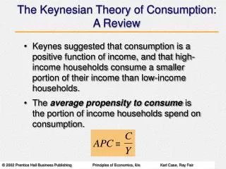
The Keynesian Theory of Consumption: A Review. Keynes suggested that consumption is a positive function of income, and that high-income households consume a smaller portion of their income than low-income households.

E N D
The Keynesian Theory of Consumption: A Review • Keynes suggested that consumption is a positive function of income, and that high-income households consume a smaller portion of their income than low-income households. • The average propensity to consume is the portion of income households spend on consumption.
The Life-Cycle Theory of Consumption • The life-cycle theory of consumption is an extension of Keynes's theory. It states that households make lifetime consumption decisions based on their expectations of lifetime income. • People tend to consume less than they earn during their main working years, and dissave during their early and later years.
The Life-Cycle Theory of Consumption • Consumption decisions are likely to be based on permanent income rather than on current income. • Permanent income is the average level of one’s expected future income stream. • Policy changes, like tax-rate changes, are likely to have more of an effect on household behavior if they are expected to be permanent rather than temporary.
The Labor Supply Decision • Households make consumption and labor supply decisions simultaneously. • Consumption cannot be considered separately from labor supply, because it is precisely by selling your labor that you earn income to pay for your consumption. • Factors that determine the quantity of labor supplied include the wage rate, prices, wealth, and nonlabor income.
The Labor Supply Decision • An increase in the wage rate causes the opportunity cost of leisure to rise, leading to a larger labor supply—a larger labor force. This is called the substitution effect of a wage rate increase. • On the other hand, a higher wage means that people will spend some of it on leisure by working less. This is the income effect of a wage rate increase. • Data suggests that the substitution effect prevails over the income effect, so higher wages lead to an increase in labor supply.
The Labor Supply Decision • Prices also play a major role in the labor supply decision. • The nominal wage rate is the wage rate in current dollars. • The real wage rate is the amount that the nominal wage rate can buy in terms of goods and services. • Workers do not care about their nominal wage—they care about the purchasing power of this wage—the real wage rate.
The Labor Supply Decision • Wealth fluctuates over the life cycle. • Holding everything else constant (including the stage in the life cycle), the more wealth a household has, the more it will consume, both now and in the future. • An unexpected increase in nonlabor income will have a positive effect on a household’s consumption. • An unexpected increase in wealth or nonlabor income leads to a decrease in labor supply.
Interest Rate Effects on Consumption • A rise in the interest rate increases the reward to saving and lowers consumption. This is the substitution effect of an interest rate change. • There is also an income effect of an interest rate change. A fall in the interest rate leads to a fall in nonlabor income and consumption.
Interest Rate Effects on Consumption • For households with positive wealth, the income effect of an interest rate change works in the opposite direction from the substitution effect. • On the other hand, if a household is a debtor, a fall in the interest rate means a fall in interest payments, so the income and substitution effects work in the same direction.
Government Effects on Consumption and Labor Supply: Taxes and Transfers
A Possible EmploymentConstraint on Households • The budget constraint, which separates those bundles of goods that are available to a household from those that are not, is determined by income, wealth, and prices. • When a household is constrained from working as much as it would like, it consumes less. • The amount that a household would like to work at the current wage rate if it could find the work is called the unconstrained supply of labor.
Keynesian Theory Revisited • It is incorrect to think consumption depends only on income, at least when there is full employment. • But if there is unemployment, the level of income depends exclusively on the employment decisions made by firms. • To the extent that Keynes emphasized the relationship between consumption and income, Keynesian theory is considered to pertain to periods of unemployment.
A Summary of Household Behavior • Factors that affect household consumption and labor supply decisions include: • current and expected future real wage rates • the initial value of wealth • current and expected future nonlabor income • interest rates • current and expected future tax rates and transfer payments
Consumption Expenditures,1970 I – 2000 II • Expenditures on services and nondurable goods are “smoother” over time than expenditures on durable goods.
Housing Investment of the Household Sector, 1970 I – 2000 II
Labor-Force Participation Rate for Men 25 to 54, Women 25 to 54, and All Others 16 and Over, 1970 I – 2000 II
Firms: Investment andEmployment Decisions • Inputs are the goods and services that firms purchase and turn into output. • There are two ways that firms can add to their stock of capital: • Plant-and-equipment investment refers to purchases by firms of additional machines, factories, or buildings within a given period. • Inventory investment occurs when a firm produces more output than it sells within a given period.
Employment Decisions • If the demand for labor increases at a time of less-than-full employment, the unemployment rate will fall. • If the demand for labor increases when there is full employment, wage rates will rise. • The demand for new capital, or planned investment spending, which is partly determined by the interest rate, is as important as the demand for labor.
Employment Decisions • The decision of how much output to produce requires a decision concerning the method of production, or technology. • A profit-maximizing firm chooses the technology that is most efficient—the one that minimizes the cost of production. • The most efficient technology depends on the relative prices of capital and labor.
Employment Decisions • A labor-intensive technology is a production technique that uses a large amount of labor relative to capital. • A capital-intensive technology is a production technique that uses a large amount of capital relative to labor. • The relative impact of an expansion of output on employment and on investment demand depends on the wage rate and the cost of capital.
Expectations and Animal Spirits • Investment decisions require looking into the future and forming expectations about it. • Expectations are always made with imperfect information. • Keynes concludes that much investment activity depends on psychology and on what he calls the animal spirits of entrepreneurs, which help to make investment a volatile component of GDP.
The Accelerator Effect • The accelerator effect is the tendency for investment to increase when aggregate output increases and decrease when aggregate output decreases, accelerating the growth or decline of output. • If aggregate output (income) (Y) is rising, investment will increase even though the level of Y may be low, further accelerating the growth of output.
Excess Labor andExcess Capital Effects • Excess labor and excess capital are labor and capital that are not needed to produce the firm’s current level of output. • Decreasing its workforce and capital stock quickly can be costly for a firm. • Adjustment costs are the costs that a firm incurs when it changes its production level—for example, the administration costs of laying off employees or the training costs of hiring new workers.
Inventory Investment Stock of inventories (end of period) = Stock of inventories (beginning of period) + Production – Sales • Inventories are counted as part of a firm’s capital stock. • The desired, or optimal, level of inventories is the level of inventory at which the extra cost (in lost sales) from lowering inventories by a small amount is just equal to the extra gain (in interest revenue and decreased storage costs).
Inventory Investment • There is a trade-off between holding inventories and changing production levels. • Because of adjustment costs, a firm is likely to smooth its production path relative to its sales path. Production should fluctuate less than sales, with changes in inventories absorbing the difference each period.
Inventory Investment • An unexpected increase in inventories has a negative effect on future production, and an unexpected decrease in inventories has a positive effect on future production. • A firm’s planned production path depends on the level of its expected future sales path. • Future sales expectations are likely to have an important effect on current production.
A Summary of Firm Behavior • The following factors affect firms’ investment and employment decisions: • the wage rate and the cost of capital. • firms’ expectations of future output. • the amount of excess labor and excess capital on hand.
A Summary of Firm Behavior • The most important points to remember about the relationship between production, sales, and inventory investment are: • inventory investment (that is, the change in the stock of inventories) equals production minus sales. • an unexpected increase in the stock of inventories has a negative effect on future production. • current production depends on expected future sales.
Plant and Equipment Investment of the Firm Sector, 1970 I – 2000 II
Inventory Investment of the Firm Sector and the Inventory/Sales Ratio, 1970 I – 2000 II
Productivity and the Business Cycle • Productivity, or labor productivity, is defined as output per worker hour (Y/H); the amount of output produced by an average worker in 1 hour. • Productivity tends to rise during expansions and fall during contractions. • During expansions, output rises by a larger percentage than employment, and the ratio of output to workers rises.
Employment and Outputover the Business Cycle • In general, employment does not fluctuate as much as output over the business cycle. • As a result, measured productivity tends to rise during expansions and decline during contractions.
Productivity in the Long Run • Theories of (long-run) economic growth focus on productivity, as measured by output per worker, or GDP per capita. • Using productivity figures to diagnose the economy in the short run can be misleading. • The tendency of firms to hold excess labor and capital, and its implications for the measurement of productivity throughout the business cycle, has nothing to do with the economy’s long-run potential to produce output.
The Relationship BetweenOutput and Unemployment • Okun’s Law is a theory put forth by Arthur Okun, that the unemployment rate decreases about one percentage point for every 3 percent increase in real GDP. • Later research and data have shown that the relationship between output and unemployment is not as stable as Okun’s “law” predicts.
The Relationship BetweenOutput and Unemployment • There are three “slippages” that combine to make the change in the unemployment rate less than the percentage change in output in the short run: • When output rises by 1 percent, the number of jobs does not tend to rise by 1 percent in the short run. • There are more jobs than there are people employed. Some of the jobs are filled by people who already have one job. • Discouraged workers move back into the labor force.
The Size of the Multiplier • There are a number of factors we have mentioned that cause the size of the multiplier to decrease. For example: • Automatic stabilizers: When the economy expands and income increases, the amount of taxes collected increases, offsetting some of the expansion. • The interest rate: All else the same, an increase in government spending causes the interest rate to increase, crowding out consumption and investment expenditures.
The Size of the Multiplier • There are a number of factors we have mentioned that cause the size of the multiplier to decrease. For example: • The response of the price level:Expansionary policy leads to an increase in the price level, which reduces the multiplier, particularly when the economy is on the steep part of the AS curve. • There are excess capital and excess labor: Output can increase by putting excess labor and capital back to work (less investment).
The Size of the Multiplier • There are a number of factors we have mentioned that cause the size of the multiplier to decrease. For example: • There are inventories: To the extent that firms draw down their inventories in the short run in response to an increase in demand, output does not respond as quickly to demand changes. • The life-cycle story and expectations: The multiplier effects for policy changes perceived to be temporary are smaller.
The Size of the Multiplier • In practice, the multiplier probably has a value of around 1.4, at its peak. For example, if government spending rises by $1 billion, then GDP rises by about $1.4 billion. • The response of the economy to a change in monetary or fiscal policy is not likely to be large and quick and, in the final analysis, the effects are much smaller than the simple multiplier would lead one to believe.