Download
1 / 23
230 likes | 547 Views
Lecture 18 Maxwell’s equations: electromagnetic waves. Introduction One of the major achievements of Maxwell was the correct prediction of electromagnetic waves from considerations of the forms of the four equations which bear his name. Maxwell’s equations

E N D
Introduction One of the major achievements of Maxwell was the correct prediction of electromagnetic waves from considerations of the forms of the four equations which bear his name.
Maxwell’s equations The general form of Maxwell’s equations (in terms of B and E), valid in the presence of dielectrics, magnetic materials, free charges and currents is:
We wish to consider the possibility of electromagnetic waves in a vacuum where there are no dielectrics, magnetic materials, free charges and currents. Hence we have JC=f=0 and r=r=1 and the form of Maxwell’s equations can be considerably simplified to:
The two RHS equations link E and B. B can be eliminated by first taking the curl of the top RHS equation where the final term is obtained by using the lower RHS Maxwell equation to eliminate B.
The next step is to simplify the initial term (E) using the identity (E)=(E)-2E but the top LHS Maxwell equation gives E=0 so (E)=-2E and hence we have finally B can also be eliminated to obtain a similar equation
The identity 2A involves the application of the Laplacian to a vector. For a scalar this gives three components, for a vector there are nine components, three for each spatial direction. For example the x-component of the resultant vector 2A has terms with similar terms for the y and z-components.
The form of the above equations for E and B is easier to see if we simplify them. For example if the y-component of the E-field (Ey) depends only on one spatial co-ordinate (e.g. x) then Ey must satisfy the equation but this is a one-dimensional wave equation that describes waves which propagate with a velocity v=(00)-½.
Worked Example Show that a function of the form represents a wave travelling along the x-axis and that it satisfies the 1D wave equation
Hence both E and B fields may exist in the forms of waves – electromagnetic waves. However if we calculate the value of (00)-½ we find it has a value equal to c, the speed of light. Hence the electromagnetic waves predicted by Maxwell’s equations propagate at the speed of light, suggesting that light itself is a form of electromagnetic radiation.
Specific properties of electromagnetic radiation The wave equations for E and B tell us that electromagnetic waves propagate at the speed of light. Further information on the form of these waves can be obtained by noting that the E- and B-fields must also satisfy Maxwell’s equations in addition to the wave equation.
We consider a specific type of wave, although the results derived are general. This wave is said to be an unbounded, plane one Plane indicates that there exist planes (or wavefronts), which are perpendicular to the direction of propagation, over which all quantities of the wave are constant. Unbounded indicates that the wave fronts can be considered to be of infinite extent.
Consider an unbounded plane wave propagating along the x-direction. The wavefronts for this wave are y-z planes. Because all quantities must be constant over a given wavefront none of the components of the E- and B-fields can be a function of yor z.
Therefore all terms with /z or /y must be zero and Maxwell’s equations become Similarly from B=0
From the above terms we immediately have therefore the components of E and B along the direction of wave propagation (x) neither vary in time or space. These components must hence be zero or at most constant and therefore can not be part of the waves. Hence for an electromagnetic wave there are no components of B and E in the direction of propagation, the wave is therefore transverse.
We now assume that the wave is polarised so that the E-field lies along the y-direction (i.e. Ey0, Ez=0). The above terms now give therefore if Eis polarised along y then B can have no component in this direction B must be polarised along z. Hence for an electromagnetic wave E, B and the direction of propagation are mutually perpendicular. A wave for which both E and B are transverse is known as a TEM wave (transverse electric and magnetic).
Finally we determine the relative sizes of E and B. As E is polarised along y and B along z we can write their spatial and temporal dependencies as (monochromatic waves): where the prefactors are constants and is a phase factor allowing for a possible phase difference between E and B. From above so
This equation can only be satisfied if =0 (i.e. E and B are in phase) and Hence at any point and time the amplitudes of Eand B are in the ratio c.
The Electromagnetic Spectrum has no limits in terms of frequency (or wavelength =c/f). • In practical terms it runs from radio waves ~103Hz to gamma waves ~1020Hz.
All frequencies obey the physics described in this lecture. • Different parts of the Electromagnetic Spectrum differ in terms of how the waves are produced, how they are deselected and the effect they have on physical and biological systems.
Conclusions • Maxwell’s equations in a vacuum and in the absence of dielectrics and magnetic materials • Derivation of the wave equations for E and B • Existence of electromagnetic waves propagating at the speed of light • Transverse nature of electromagnetic waves • Relationship between amplitudes of E and B