Download

1 / 34
380 likes | 668 Views
10. Frequency Response Analysis (I). Yonsei University Mechanical Engineering Prof. Hyun Seok YANG. * Frequency Response is the steady state response of a (linear) system to a sinusoidal input. (Linear) System. Dynamic behavior of the system in frequency domain - Bandwidth

E N D
10. Frequency Response Analysis (I) Yonsei University Mechanical Engineering Prof. Hyun Seok YANG
* Frequency Response is the steady state response of a (linear) system to a sinusoidal input. (Linear) System Dynamic behavior of the system in frequency domain - Bandwidth - System behavior to noise and disturbance - Relative stability c.f > Root Locus Analysis - Transient response (rise time, settling time, %OS, etc.)
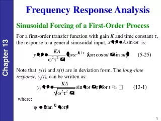
: Magnitude Ratio : Phase Angle Output Frequency = Input Frequency : Sinusoidal Transfer Function
? [Example]
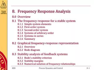
(1) Logarithmic Plot (Bode Plot) * Magnitude v.s. * Phase Angle v.s. (2) Polar Plot (Nyquist Plot) (3) Log-Mag v.s. Phase Plot (Nichols Chart) * Graphical Representation of Frequency Response Magnitude & Phase
[dB : Decibel] The magnitudes & phase angles of the system are the sum of those of each sub-components, respectively. Therefore, in order to get the total mag. & angle, all we need is just to add them up. BODE PLOT <e.g.>
For K>0 (a)
[Differentiator] - 20 dB/dec + 20 dB/dec (b) [(Free) Integrator]
Break Freq. - 20 dB/dec - 20 dB/dec (c)
Figure 10.8 Asymptotic and actual normalized and scaled response of (s + a)
Figure 10.9 Normalized and scaled Bode plots for a. G(s) = s; b. G(s) = 1/s; c. G(s) = (s + a); d. G(s) = 1/(s + a)
Figure 10.16 Normalized and scaled response for
Figure 10.14 Normalized and scaled response for
- 20 dB/dec - 60 dB/dec [Example]
1 2 4 3 [Example]
[Note] At high frequency : * For minimum phase system (i.e. no poles or zeros in RHP) - Slope of Mag. Plot @ = - 20 dB/dec x (# poles - # zeros) - Phase Angle = - 900 x (# poles - # zeros) * For non-minimum phase system (i.e. at least one poles or zeros in RHP) - Slope of Mag. Plot @ = - 20 dB/dec x (# poles - # zeros) - Phase Angle = - 900 x (# poles - # zeros)
* All three have the same mag. plot. * All three have different phase angle plots. [Non-minimum phase system Bode Plot] [Example]
[System Identification using Bode Plot] Unknown Linear Sys 1) Apply sinusoid input for wide range of input frequencies and mark mag. ratios & phase angles on the Bode plot. 2) Draw an asymptotic line based on the marks. 3) Find break frequencies. 4) Determine whether the sytem is min or non-min phase, base on the slope of the mag. ratio & phase angle. 5) Find the DC Gain. [Note] There are many H/W & S/W tools to do the above procedures. (e.g. Dynamics Signal Analyzer, FFT Analyzer)
Extended line of - 20 dB/dec - 60 dB/dec - 40 dB/dec - 40 dB/dec
[Example] Identification of VCM Actuator Dynamics Experimental Setup for VCM FRF(Bode Plot) Position FRF result at slider
[Note] [original signal] [noise] [signal with noise]
[the original signal after noise is eliminated.] [signal with noise] • Above from which freq will be filtered out should be determined • carefully. [The choice of ] • * Phase Delay problem should also be considered.
* Polar Plot of a sinusoidal transfer function - Locus of vectors in complex plane for [Example] NYQUIST PLOT
+ + [Nyquist Stability Criterion] Recall * Characteristic Equation
which lie inside some closed contour in S-plane. [i.e. Contour does not pass through any poles or zeros of F(s).] S-plane Im F-plane Mapping Re Mapping Theorem [Note] C.W direction : + Let N be the total # of C.W. encirclements of the origin of F-plane Then, z = N + p
S-plane Im F-plane Nyquist Path Mapping Re # of Unstable C.L. Poles # of Unstable O.L. Poles * Nyquist Path Then, since z = N + p
F-plane -1 Nyquist Plot of O.L.T.F. [Note] Im Im GH -plane F-plane semi-circle contour with infinite radius maps into a point in GH (or F)-plane. Mapping Re Re S-plane a point Only need to examine the contour on jw-axis By the way, 0
Nyquist Stability Criterion For a C.L. system to be stable, “z” should be zero. “z = N + p” means (from Nyquist plot of O.L.T.F.) z = # of Unstable C.L. Poles N = # of C.W. Encirclements of (-1+0j) Point of Nyquist Plot of O.L.T.F. p = # of Unstable O.L. Poles [Note] When the locus of GH passes through (-1+0j) point, then the C.L. poses are located on the jw-axis.
[Example] S-plane 3 4 1 1 2 [Note] When G(s)H(s) has poles or zeros on the jw-axis, modify the Nyquist path not to pass through those poles or zeros.
3 2
Im Symmetric on the Re-axis with Re 4 4 4 1 [Nyquist Plot] 3 2 2
<K small> Im <K large> Im Re Re -1 -1 z = 2 Untable z = 0 Stable <c.f.> Root Locus [Example] Nyquist Stability Criterion p = 0, N = 2 p = 0, N = 0