Download
1 / 35
350 likes | 641 Views
Travel Cost Modeling: The Value of Enhanced Water Levels at Walker Lake to Recreational Users. presented by W. Douglass Shaw Texas A&M. The Problem - Background. Walker Lake is a terminus lake in Great Basin fed by Walker River, a winter sport fishery

E N D
Travel Cost Modeling: The Value of Enhanced Water Levels at Walker Lake to Recreational Users presented by W. Douglass Shaw Texas A&M
The Problem - Background • Walker Lake is a terminus lake in Great Basin • fed by Walker River, a winter sport fishery • Walker is “dying” – 140 foot decline since 1882 • TDS levels have increased from 2500 mg/L in 1882 to 13,300 mg/L in 1994 • Can something be done to restore lake levels, or at least halt the decline?
Why Care? -- Fish Survival • Fish cannot survive above 16,000 mg/L of TDS • Corresponds to about a 2.3 million acre feet critical level (about the level at end of 1997) • fell below this in 1992 • will hit critical level within 20? years
Recent Concerns • TDS in January, 2004 already at 15,300 ppm • Loons feed on Tui Chub • Tui Chub stopped reproducing in 2003 • Upstream Tamarisk problem (one tree, up to 200 gallons per day)
Project Originally Funded by U.S. Bureau of Reclamation • Data Collection: 1995-1996 • Tie to Potential for Regional Water Bank • Elizabeth Fadali, MS from UNR (thesis), two students in hydro from DRI • Additional work in 1999 by Mark Eiswerth, UNR • More work in 2000 with Frank Lupi, MSU
Aside: Water Banks • Existing Water Banks in Idaho, California, New Mexico, Texas • state run • deposits from farmers and ranchers • withdrawals by cities, industry • California’s most active in drought periods
Supply and Demand • Supply is typically the Agricultural sector, with most of the water • Demand is typically the demand by hyrdo-electric power producers or recreation or environmental groups
Focus: Recreational Use • Uses Travel Cost/ Recreation Demand Models • New Feature Today: Contingent Behavior Modeling • What would you do if… • No Inclusion of "Non-use" or Passive Use Values
Travel Cost Models • Review: • Q = f(P,Z), where Q is the trip, P is the trip “price” and Z are other variables that influence the number of trips, such as the destination’s quality • Old models: Estimate Q = a – bP + cZ using ordinary least squares
Consumer’s Surplus and TCM • Using the predicted demand function, calculate the area under the demand curve as “ordinary” consumer’s surplus or Marshallian welfare • More modern approach: calculate “Hicksian” welfare measures/exact consumer’s surplus
Exact CS • Define the compensating variation (CV) for price decrease to P’’: • V(P’,Y) = V(P’’,Y – CV), where V is the indirect utility function, Y is income • Define the equivalent variation (EV) for a price decrease to P’’ • V(P’, Y + EV) = V(P’’,Y)
Interpretation • CV – the amount of money that must be taken away at the new price level, such that the person is indifferent between the original prices and the new (property right is NOT with the individual – holds him at the original - WTP) • EV – amount of money individual must be compensated with to forgo the change (property right IS with the individual - WTA)
Income Effects • If income effects exist, there is a price and income effect (price decrease generates additional “income” – but we wish to hold that effect constant) • Most valuation models have no income effects, so CV = EV = Ordinary CS
Y Price decrease in X b a U1 Uo X
Surveys • Very Small Recreation Research Budget • Good-Sized "Intercept" Sample (N = 573) • Yields Biased Sample of Recreational Users
On-Site Surveys • Send student crew to region lakes in 1995 and 1996, in summer only • Lots of effort at Lahonton, Pyramid, not just Walker Lake • Why biased sample?
Biased sample • On-site (not all seasons) • people who are more avid, more likely to be surveyed (higher probability of being intercepted) • maybe their preferences for lakes are stronger • not like the general public • Pyramid and Walker are winter fisheries
Innovations (statistics) • The random utility model and the count data model • Demand systems (non-normally distributed trips)
Application of Random Utility Model • Conventional multinomial logit (conditional on trips being fixed for the season):
RUM Results • Fadali and Shaw, 1998 (Contemporary Economic Policy) - uses RP data only for Five Lakes • Mean WTP to Prevent "Elimination" $83 per season/person • Adjustments: Use Non-visitor WTP of only $8 per season • Total Annual Value: About $4 million • Conclusion: Demand/value large enough to rent significant amounts of water from Ag Sector
Shortcomings of Original Study • Biased Sample leads to needed adjustments • No exact modeling of impacts of specific water level changes on angling and other users • Model may fail to predict “out of sample” results
Some New Results • See Eiswerth et al. 2000 (Water Resources Research) • Uses Contingent Behavior Data, Walker Lake Only • Scenarios: 20 foot increase/decline in lake level tied to Thomas (U.S.G.S., 1995) • Support of "convergent validity" -- RP and CB data are consistent
Contingent Behavior • Not CVM, rather: • “Presume water levels rise by 20 feet at Walker Lake with changed programs. Would you take more/fewer trips to Walker Lake? Elsewhere? • If yes, how many more/fewer?
Count Data Model • Trips (qji) are not normally distributed • They cannot be negative • They typically take integer values • They can be zero (unless doing an intercept) • They usually cannot exceed a value of about 200 (day trips)
Count Model/Contingent Behavior Results • Mean WTP for a "trip" $88 • Values for a 1 foot increase, per person $12 - $18/yr • Values for 20 foot increase $240 - $360 /person/yr • Totals for 20 foot increase: About $7 million to $13.5 per year
Some Even Newer Results • See Fadali, Lupi and Shaw (2004) • Formal Statistical Adjustment for Biased Sample • Mean WTP compared to Fadali and Shaw drops significantly • WTP’s for general and on-site sample differ • On-site per trip WTP to prevent elimination of Walker: $9.85 vs. “general” of $2.63