Download
1 / 46
470 likes | 556 Views
Statistical Analysis of DNA Microarray. An Example of HDLSS in Genetics. The Data. Expression Matrix. Rows represent genes = feature vectors. Columns represent different cell samples. Ex: cancer cells from different patients.

E N D
Statistical Analysis of DNA Microarray. An Example of HDLSS in Genetics.
ExpressionMatrix • Rows represent genes = feature vectors. • Columns represent different cell samples. Ex: cancer cells from different patients. • Each element (i,j) of the array represents the expression level of genei in cell sample j.
Goal of Analysis of Expression Matrix • Some statistical methods applied to: • “Group” similar genes together => groups of functionally similar genes. • “Extract” representative gene in each group. • ”Group” similar cell samples together.
Overview DNA Microarray Technology • One cell sample. • Level of expression. • Microarray technique.
Getting the Data…measuring the Level of Expression Gene by Gene. • Each spot in this DNA microarray represents the level of expression of a single gene in the tumor cell compared to a reference cell. • Standardize the level of expression of this cell to make it comparable to other cells. Expressed in reference cell. Expressed in reference and tumor cell. Expressed in tumor cell Nor expressed.
Level of Expression …mRNA • All the cells contain the same DNA = same genes, but in one cell not all genes are active. • What differentiate the cells is what genes are active or expressed. • To measure the cell expression we measure the genetic molecule “RNA messenger” denoted by mRNA.
RNAm is one strand copy of a piece of DNA. Highly unstable. DNA is double stranded, one strand complementary to the other. Stable. RNAm … DNA
Microarray Technique (Cont.)…The Microarray Microarrays are made from a collection of purified DNA's. A drop of each type of DNA in solution is placed onto a specially-prepared glass microscope slide by an arraying machine. The arraying machine can quickly produce a regular grid of thousands of spots in a square about 2 cm on a side, small enough to fit under a standard slide coverslip. The DNA in the spots is bonded to the glass to keep it from washing off during the hybridization reaction
Microarray Technique (Cont.) …Description of the Method • Definition of Microarray from the National Human Genome Research Institute : “…The method uses a robot to precisely apply droplets containing functional DNA to glass slides. Researchers then attach fluorescent labels to DNA from the cell they are studying. The labeled probes are allowed to bind to complementary DNA strands on the slides. The slides are put into a scanning microscope that can measure the brightness of each fluorescent dot; brightness reveals how much of a specific DNA fragment is present, an indicator of how active it is.”
Microarray Technique (Cont.) …The Method Step by Step • First step : to measure the gene expression level of a cell, collect RNAm from the cell of interest, usually cancer cell. Have the same quantity of RNAm from a “reference cell”. • Second step: RNAm to cDNA. The RNAm is highly unstable, to stabilize it we complement the strand and create cDNA(complementary DNA) . • Third step: creates cDNA probes. Label cDNA from each cell by fluorescent dyes. A differently colored fluor is used for each sample.
Microarray Technique …The Method Step by Step (Contd.) • Fourth step: hybridize the cDNA probes from the two samples to the Microarray. Once the cDNA probes have been hybridized to the array and any loose probe has been washed off, the array must be scanned to determine how much of each probe is bound to each spot.
Statistical Methods • Clustering. • Gene shaving algorithm: use of PCA for clustering.
Clustering Overview - Kmean clustering. - Hierarchical clustering. - Validation method.
What Is Clustering? • For a sample of size ndescribed by a d-dimensional feature space,Clustering is a procedure that: • . Divide the d-dimensional feature space in k disjoint groups. • . Data points within each group are moresimilar to each other than to any data point in other groups. Illustration for n = 45, d = 2 andk = 3.
Similarity Between Feature Vectors • Choice of the similarity function depends on the data. For example: if data is invariant by linear transformation or rotation than the similarity function has to be invariant too. Similarity function could be a distance or an inner product. • Examples of similarity functions: • Euclidean distance, used to illustrate for d = 2. • Correlation is used for microarray data.
K-means Clustering • Divide the d dimensional feature space on “k” parts described by Voronoi partition of the k mean vectors. • Algorithm finds the vector of means of clusters. Illustration for d =2 and k = 3, red points represent means of clusters and red lines represent Voronoi partition.
Algorithm Begininitializen, k, m1, m2,..., mk Do classify nsamples according to nearestmi recomputemi until no change in mi returnm1, m2,..., mk end Computational ComplexityO(ndkT) Tis the number of iterations Algorithm for K-means Clustering For d = 2, illustration of the trajectories of the 3 means.
K-mean Clustering for Microarray Data • Cf picture k.mean. • K-means clustering of lymphoma data. Lymphoma profiles were clustered using the expression of 148 germinal-center-specific genes and Euclidean distance metric.(a) represents the germinal-cell subtype; and (b) represents the activated subtype. Each column represents a specific gene and each row a specific cancer profile.
Hierarchical Clustering Venn Diagram of Clustered Data Dendrogram
Hierarchical Clustering (Cont.) • Multilevel clustering, at level 1 we have n clusters and at level n we have one cluster. • Agglomerative HC: starts with singleton and merge clusters. • Divisive HC :starts with one sample and split clusters.
Hierarchical Clustering …NearestNeighborAlgorithm • Nearest Neighbor Algorithm is an agglomerative HC (bottom-up). • The algorithm starts with n nodes (n is the size of our sample). At every level the 2 most similar nodes are merged together into one node. The algorithm stops when we get the desired number of clusters.
Results of Hierarchical Clustering on Microarray Data • Grouping similar functional genes. • Grouping similar cell samples. • Cf picture Perou.trend.review2001.pdf file page6.
Criterion Function for Clustering • Criterion Functions depend on grouping and number of clusters. Examples are: • Sum of squared errors || x - mi || 2. • Scatter Criteria |SW| / |ST| ; where ST=SW+SB . i.e. decompose the total scatter matrix into between-cluster scatter matrix and within-cluster scatter matrix. • Best cluster minimizes the criterion.
Gene Shaving • The “gene shaving” method is also a method of clustering genes and sample cells. But unlike classic clustering, in this method one gene could belong to more than one cluster.
1. Start with the entire expression matrix X, each row centered to have zero mean. 2. Compute the leading PC of the rows of X. 3. Shave off the proportion alpha (10%) of the genes having smallest absolute inner-product with the leading PC. 4. repeats steps 2 and 3 until only one gene remains. 5. This produces a nested sequence of gene clusters Sn... Sk … S 1 where Sk denotes a cluster of kgenes. Estimates the optimal cluster size kusing the gap statistic. 6. Orthogonalize each row of X with respect to Sk , the average gene in Sk , optimal from step5. 7. Repeat steps 1-5 with orthogonalized data, to find the second optimal cluster. This process continued until a max of M clusters are found. Gene Shaving…iteration
To Estimate Cluster Size : Gap Estimate • For cluster Sklet Dkbe the scatter estimate. i.e Dk = 100 SB/ST. • For b in {1,…,B}, let • X * (b)permuted data matrix ( permuting the elements within each row of X ). • Dk* (b) is the scatter estimate for cluster Sk *(b). • Dk*is the mean of Dk* (b)’s. • Gap(k) = Dk - Dk* . • Choose k that produces the largest gap.
Gene Shaving (Cont.) The first three gene clusters found for the DLCL data
Gene Shaving (Cont.) Percent of gene variance explained by first j gene shaving column averages (j = 1,2,... 10) (solid curve), and by first j principal components (broken curve). For the shaving results, the total number of genes in the first j clusters is also indicated.
Gene Shaving ( Cont.) a) Variance plots for real and randomized data. The percent variance explained by each cluster, both for the original data, and for an average over three randomized versions. (b) Gap estimates of cluster size. The gap curve, which highlights the difference between the pair of curves, is shown.
References • Pattern Classification Richard O.Duda, Peter E.Hart and David G.Stork Chapter 10. • ‘Gene Shaving’ as a method for identifying distinct sets of genes with similar expression patterns T. Hastie, R. Tibshirani, M.B. Eisen, A Alizadeh, R. Levy,L Staudt, W.C Chan, D.Botstein and P. Brown. Genome Biology 2000. http://genomebiology.com/2000/1/2/research/0003/#B14. • Cluster analysis and display of genome-wide expression patterns, PNAS (1998).
References • Basic microarray analysis: grouping and feature reduction. S. Raychaudhuri, P.Sutphin, J.T. Chang and Russ B. Trends in Biotechnology 2001. • Tumor classification using gene expression patterns from DNA microarrays.Charles M. Perou, Patrick O.Brown and David Botstein. Trends in Molecular medicine ,December 2000. • Pictures and definition of microarray technology from National Human Genome Research Institute