Download
1 / 34
360 likes | 614 Views
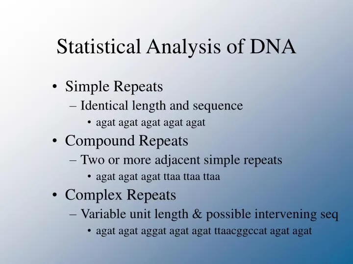
Statistical Analysis of DNA. Simple Repeats Identical length and sequence agat agat agat agat agat Compound Repeats Two or more adjacent simple repeats agat agat agat ttaa ttaa ttaa Complex Repeats Variable unit length & possible intervening seq

E N D
Statistical Analysis of DNA • Simple Repeats • Identical length and sequence • agat agat agat agat agat • Compound Repeats • Two or more adjacent simple repeats • agat agat agat ttaa ttaa ttaa • Complex Repeats • Variable unit length & possible intervening seq • agat agat aggat agat agat ttaacggccat agat agat
STR NOMENCLATURE • Microvariants • Alleles that contain incomplete units • TH01 9.3 • aatg aatg aatg aatg aatg aatg aatg aatg aatg aatg - 10 • aatg aatg aatg aatg aatg aatg atg aatg aatg aatg - 9.3
STRs Used In Forensic Science • Need lots of variation - polymorphic • Overall short segments - 100-400 bp • Can use degraded DNA samples • Segment size usually limits preferential amplification of smaller alleles • Single base resolution • TH01 9.3 • TETRANUCLEOTIDE REPEATS • Narrow allele size range - multiplexing • Reduces allelic dropout (stochastic effects) • Use with degraded DNA possible • Reduced stutter rates - easier to interpret mixtures
ALLELIC LADDERS • Artificial mixture of common alleles • Reference standards • Enable forensic scientists to compare results • Different instruments • Different detection methods • Allele quantities balanced • Produced with same primers as test samples • Commercially available in kits
Profiler Plus Allelic Ladders VWA D3S1358 FGA AMEL D8S1179 D21S11 D18S51 D13S317 D5S818 D7S820
PCR Product Size (bp) D3S1358 vWA FGA Power of Discrimination Blue 1:5000 1:410 1:3.6 x 10⁹ 1:9.6 x 10¹⁰ 1:8.4 x 10⁵ 1:3.3 x 10¹² TH01 CSF1PO TPOX Amel Green I TH01 D13S317 D3S1358 CSF1PO vWA TPOX FGA Amel D5S818 D7S820 Profiler D8S1179 D13S317 Amel vWA D7S820 D3S1358 D5S818 D21S11 FGA Profiler Plus D18S51 TH01 D7S820 D3S1358 TPOX CSF1PO Amel COfiler D16S539 D3S1358 vWA Amel D8S1179 D18S51 TH01 D16S539 D21S11 D19S433 D2S1338 SGM Plus FGA Same DNA Sample Run with Each of the ABI STR Kits
STR LOCI ALLELES • TPOX • THYROID PEROXIDASE • Chromosome 2 • AATG repeat • 6 to 13 repeats • TH01 • TYROSINE HYDROXYLASE • Chromosome 11 • TCTA repeat (Bottom strand) • 4 to 11 repeats • Common microvariant 9.3
STR LOCI ALLELES • vWA • von Willebrand Factor • Chromosome 12 • TCTA with TCTG repeat • 10 to 22 repeats • D3S1358 • Chromosome 3 • AGAT with AGAC repeat • 12 to 20 repeats
13 CODIS Core STR Loci with Chromosomal Positions TPOX D3S1358 TH01 D8S1179 D5S818 VWA FGA D7S820 CSF1PO AMEL D13S317 AMEL D16S539 D18S51 D21S11
Position of Forensic STR Markers on Human Chromosomes TPOX D3S1358 TH01 D8S1179 D5S818 VWA FGA D2S1338 D7S820 CSF1PO AMEL Sex-typing Penta E D19S433 D13S317 AMEL D16S539 D18S51 D21S11 Penta D 13 CODIS Core STR Loci
45 40 35 30 Caucasians (N=427) 25 Frequency Blacks (N=414) 20 Hispanics (N=414) 15 10 5 0 6 7 8 9 9.3 10 Number ofrepeats STR Allele FrequenciesExclusions don’t require numbers Matches do require statistics TH01 Marker *Proc. Int. Sym. Hum. ID (Promega) 1997, p. 34
A1A1 A1A2 A2A2 A1 A2 p1p2 A1 A1A1 A1A2 p1p2 A2 A1A2 A2A2 Hardy - Weinberg Equilibrium frequency at one locus p12 2p1p2 p22 p12 freq(A1) = p1 p22 freq(A2) = p2 (p1 + p2 )2 = p12 + 2p1p2 + p22
Product Rulefrequency at one locus • The frequency of a multi-locus STR profile is the product of the genotype frequencies at the individual loci ƒ locus1 x ƒ locus2 x ƒ locusn = ƒcombined Criteria for Use of Product Rule • Inheritance of alleles at one locus have no effect on alleles inherited at other loci
ProfIler Plus Item D3S1358 vWA FGA D8S1179 D21S11 D18S51 D5S818 D13S317 D7S820 Q1 16,16 15,17 21,22 13,13 29,30 16,20 8,12 12,12 8,11 CoFIler Item D3S1358 D16S539 TH01 TPOX CSF1P0 D7S820 Q1 16,16 10,12 8,9.3 9,10 12,12 8,11
D3S1358 = 16, 16 (homozygote) Frequency of 16 allele = ??
D3S1358 = 16, 16 (homozygote) Frequency of 16 allele = 0.3071 When same allele: Frequency = genotype frequency (p2) Genotype freq = 0.3071 x 0.3071 = 0.0943 This is the random match probability
ProfIler Plus Item D3S1358 vWA FGA D8S1179 D21S11 D18S51 D5S818 D13S317 D7S820 Q1 16,16 15,17 21,22 13,13 29,30 16,20 8,12 12,12 8,11 CoFIler Item D3S1358 D16S539 TH01 TPOX CSF1P0 D7S820 Q1 16,16 10,12 8,9.3 9,10 12,12 8,11
VWA = 15, 17 (heterozygote) Frequency of 15 allele = ?? Frequency of 17 allele = ??
VWA = 15, 17 (heterozygote) Frequency of 15 allele = 0.2361 Frequency of 17 allele = 0.1833 When heterozygous: Frequency = 2 X allele 1 freq X allele 2 freq (2pq) Genotype freq = 2 x 0.2361 x 0.18331 = 0.0866 Overall profile frequency = Frequency D3S1358 X Frequency vWA 0.0943 x 0.0866 = 0.00817 This is the combined random match probability
Population database • Look up how often each allele occurs at the locus in a population (the “allele” frequency)
13 14 15 16 17 18 19 20 13 0 0 0 1 0 0 1 0 14 1 4 10 10 10 4 0 153 7 14 8 4 1 16 11 27 7 3 1 17 11 23 8 1 18 16 6 0 19 3 1 20 0 0 Frequency of allele 13 = [(1 + 1)/(196*2)] x 100 = 0.510% i.e. total # of occurrences / total # of alleles Frequency of allele 15 = [(4+6+7+14+8+4+1)/(196*2)] x 100 = 11.224% i.e. total # of occurrences / total # of alleles NOTE: for the case of the homozygous occurrence (16,16) the frequency of allele 16 is twice the number of individual observations
Match probability (MP) is calculated as the square frequency of the most common allele to provide the most conservative estimate of a random match for a given individual. The power of discrimination (PD) is one minus MP. MP= (.26276)2= .069 PD= (1-0.069) = .931
Heterozygosity is also called the frequency of heterozygotes and is represented by h in the following equation. Where nh is the number of individual observations with two alleles and n is the total number of individuals. Since one is either a homozygote or a heterozygote, the frequency of heterozygotes (h) plus the frequency of homozygotes (H) is equal to one. The power of exclusion, PE, is defined as the probability of excluding a random individual from the population as a potential parent based on the genotype of one parent and offspring,. The average for a given locus is represented by the following equation: The greater the heterozygosity (h), the greater the value of PE, and the greater the effectivenness of this locus as a means of excluding a random individual from the population as a potential parent of a given individual.
h= 151/196 = .7704 H= (1-0.7704) = .2296 PE = (.77)2x(1-2x.7704x[.2296]2) PE = 0.545 Note difference
A A A B B A AB AA AB AB C C AC AC AC BC The greater the heterozygosity (h), the greater the value of PE, and the greater the effectivenness of this locus as a means of excluding a random individual from the population as a potential parent of a given individual. The more heterozygous allele distribution gives less variable allele distribution for offspring, allowing us to exclude more individuals as potential parents. Can exclude everyone except carriers of allele A
0.005 0.102 0.112 0.201 0.263 0.222 0.084 0.010 0.005 0.005 0.200 0.220 0.394 0.515 0.435 0.165 0.020 0.102 2.039 4.478 8.037 10.516 8.876 3.359 0.400 0.112 2.459 8.825 11.547 9.747 3.688 0.439 0.201 7.919 20.722 17.492 6.619 0.788 0.263 13.557 22.887 8.660 1.031 0.222 9.660 7.310 0.870 0.084 1.383 0.329 0.010 0.020 From the observed allele frequencies that we have just calculated a table of expected observations is calculated. Each entry is calculated as the allele frequency for that pair but the result must then multiplied by the total number of individuals When heterozygous: 2 x (allele 1 freq) x ( allele 2 freq) x N = (2pq) x 196 When homozygous: (allele freq)2 x N = (p)2 x 196
h= 158.96/196 = .811 H= (1-0.811) = .189 PE = (.811)2x(1-2x.811x[.189]2) PE = 0.611
The c2 test first calculates a c2 statistic using the formula: where: Aij = actual frequency in the i-th row, j-th column Eij = expected frequency in the i-th row, j-th column r = number or rows c = number of columns A low value of c2 is an indicator of independence. As can be seen from the formula, c2 is always positive or 0, and is 0 only if Aij = Eij for every i,j. CHITEST returns the probability that a value of the c2 statistic at least as high as the value calculated by the above formula could have happened by chance under the assumption of independence. To find the c2 statistic value for the reported value of p: Step 1.Select a cell in the work sheet, the location which you like the CHI-SQUARE statistic to appear. Step 2. From the menus, select insert then click on the Function option, Paste Function dialog box appears. Step 3.Refer to function category box and choose statistical, from function name box select CHIINV and click on OK. Step 4.When the CHIINV dialog appears: Enter the cell containing the p-value (0.9798) and then enter 28 for the degrees of freedom , and finally click on OK. A value of 14.98 is returned, and this is equal to the c2 statistic
We now have a table of observed and a table of expected values. To compare the observed values with the expected values a a CHI-SQUARE test is performed In EXCEL . Step 1.Select a cell in the work sheet, the location which you like the p value of the CHI-SQUARE to appear. Step 2. From the menus, select insert then click on the Function option, Paste Function dialog box appears. Step 3.Refer to function category box and choose statistical, from function name box select CHITEST and click on OK. Step 4.When the CHITEST dialog appears: Enter the actual-range and then enter the expected-range , and finally click on OK. The p-value will appear in the selected cell. Since the p-value of 0.9798 is greater than the level of significance (0.05), it fails to reject the null hypothesis. This verifies the independence of the alleles, as well as indicating that the the sample used is not statistically different from the general population.