Download
1 / 25
280 likes | 401 Views
R-Trees: A Dynamic Index Structure For Spatial Searching Antonin Guttman. Introduction. Range queries in multiple dimensions: Computer Aided Design (CAD) Geo-data applications Support spacial data objects (boxes) Index structure is dynamic. R-Tree. Balanced (similar to B+ tree)

E N D
R-Trees: A Dynamic Index Structure For Spatial SearchingAntonin Guttman
Introduction • Range queries in multiple dimensions: • Computer Aided Design (CAD) • Geo-data applications • Support spacial data objects (boxes) • Index structure is dynamic.
R-Tree • Balanced (similar to B+ tree) • I is an n-dimensional rectangle of the form (I0, I1, ... , In-1) where Ii is a range [a,b] [-,] • Leaf node index entries: (I, tuple_id) • Non-leaf node entry: (I, child_ptr) • M is maximum entries per node. • m M/2 is the minimum entries per node.
Invariants • Every leaf (non-leaf) has between m and M records (children) except for the root. • Root has at least two children unless it is a leaf. • For each leaf (non-leaf) entry, I is the smallest rectangle that contains the data objects (children). • All leaves appear at the same level.
Searching • Given a search rectangle S ... • Start at root and locate all child nodes whose rectangle I intersects S (via linear search). • Search the subtrees of those child nodes. • When you get to the leaves, return entries whose rectangles intersect S. • Searches may require inspecting several paths. • Worst case running time is not so good ...
Insertion • Insertion is done at the leaves • Where to put new index E with rectangle R? • Start at root. • Go down the tree by choosing child whose rectangle needs the least enlargement to include R. In case of a tie, choose child with smallest area. • If there is room in the correct leaf node, insert it. Otherwise split the node (to be continued ...) • Adjust the tree ... • If the root was split into nodes N1 and N2, create new root with N1 and N2 as children.
Adjusting the tree • N = leaf node. If there was a split, then NN is the other node. • If N is root, stop. Otherwise P = N’s parent and EN is its entry for N. Adjust the rectangle for EN to tightly enclose N. • If NN exists, add entry ENN to P. ENN points to NN and its rectangle tightly encloses NN. • If necessary, split P • Set N=P and go to step 2.
Deletion • Find the entry to delete and remove it from the appropriate leaf L. • Set N=L and Q = . (Q is set of eliminated nodes) • If N is root, go to step 6. Let P be N’s parent and EN be the entry that points to N. If N has less than m entries, delete EN from P and add N to Q. • If N has at least m entries then set the rectangle of EN to tightly enclose N. • Set N=P and repeat from step 3. • *Reinsert entries from eliminated leaves. Insert non-leaf entries higher up so that all leaves are at the same level. • If root has 1 child, make the child the new root.
Why Reinsert? • Nodes can be merged with sibling whose area will increase the least, or entries can be redistributed. • In any case, nodes may need to be split. • Reinsertion is easier to implement. • Reinsertion refines the spatial structure of the tree. • Entries to be reinserted are likely to be in memory because their pages are visited during the search to find the index to delete.
Other Operations • To update, delete the appropriate index, modify it, and reinsert. • Search for objects completely contained in rectangle R. • Search for objects that contain a rectangle. • Range deletion.
Splitting Nodes • Problem: Divide M+1 entries among two nodes so that it is unlikely that the nodes are needlessly examined during a search. • Solution: Minimize total area of the covering rectangles for both nodes. • Exponential algorithm. • Quadratic algorithm. • Linear time algorithm.
Splitting Nodes – Exhaustive Search • Try all possible combinations. • Optimal results! • Bad running time!
Splitting Nodes – Quadratic Algorithm • Find pair of entries E1 and E2 that maximizes area(J) - area(E1) - area(E2) where J is covering rectangle. • Put E1 in one group, E2 in the other. • If one group has M-m+1 entries, put the remaining entries into the other group and stop. If all entries have been distributed then stop. • For each entry E, calculate d1 and d2 where di is the minimum area increase in covering rectangle of Group i when E is added. • Find E with maximum |d1 - d2| and add E to the group whose area will increase the least. • Repeat starting with step 3.
Greedy continued • Algorithm is quadratic in M. • Linear in number of dimensions. • But not optimal.
Splitting Nodes – Linear Algorithm • For each dimension, choose entry with greatest range. • Normalize by dividing the range by the width of entire set along that dimension. • Put the two entries with largest normalized separation into different groups. • Randomly, but evenly divide the rest of the entries between the two groups. • Algorithm is linear, almost no attempt at optimality.
Performance Tests • CENTRAL circuit cell (1057 rectangles) • Measure performance on last 10% inserts. • Search used randomly generated rectangles that match about 5% of the data. • Delete every 10th data item.
With linear-time splitting, inserts spend very little time doing splits. • Increasing m reduces splitting (and insertion) cost because when a groups becomes too full, the rest of the entries are assigned to the other group. • As expected, most of the space is taken up by the leaves.
Deletion cost affected by size of m. For large m: • More nodes become underfull. • More reinserts take place. • More possible splits. • Running time is pretty bad for m = M/2. • Search is relatively insensitive to splitting algorithm. Smaller values of m reduce average number of entries per node, so less time is spent on search in the node (?).
Space Efficiency • Stricter node fill produces smaller index. • For very small m, linear algorithm balances nodes. Other algorithms tend to produce unbalanced groups which are likely to split, wasting more space.
Conclusions • Linear time splitting algorithm is almost as good as the others. • Low node-fill requirement reduces space-utilization but is not siginificantly worse than stricter node-fill requirements. • R-tree can be added to relational databases.