Download
1 / 66
720 likes | 891 Views
R-Trees: A Dynamic Index Structure For Spatial Searching Antonin Guttman. Introduction. Range queries in multiple dimensions: Computer Aided Design (CAD) Geo-data applications Support spacial data objects (boxes) Index structure is dynamic. R-Tree. Balanced (similar to B+ tree)

E N D
R-Trees: A Dynamic Index Structure For Spatial SearchingAntonin Guttman
Introduction • Range queries in multiple dimensions: • Computer Aided Design (CAD) • Geo-data applications • Support spacial data objects (boxes) • Index structure is dynamic.
R-Tree • Balanced (similar to B+ tree) • I is an n-dimensional rectangle of the form (I0, I1, ... , In-1) where Ii is a range [a,b] [-,] • Leaf node index entries: (I, tuple_id) • Non-leaf node entry: (I, child_ptr) • M is maximum entries per node. • m M/2 is the minimum entries per node.
Invariants • Every leaf (non-leaf) has between m and M records (children) except for the root. • Root has at least two children unless it is a leaf. • For each leaf (non-leaf) entry, I is the smallest rectangle that contains the data objects (children). • All leaves appear at the same level.
Searching • Given a search rectangle S ... • Start at root and locate all child nodes whose rectangle I intersects S (via linear search). • Search the subtrees of those child nodes. • When you get to the leaves, return entries whose rectangles intersect S. • Searches may require inspecting several paths. • Worst case running time is not so good ...
Insertion • Insertion is done at the leaves • Where to put new index E with rectangle R? • Start at root. • Go down the tree by choosing child whose rectangle needs the least enlargement to include R. In case of a tie, choose child with smallest area. • If there is room in the correct leaf node, insert it. Otherwise split the node (to be continued ...) • Adjust the tree ... • If the root was split into nodes N1 and N2, create new root with N1 and N2 as children.
Adjusting the tree • N = leaf node. If there was a split, then NN is the other node. • If N is root, stop. Otherwise P = N’s parent and EN is its entry for N. Adjust the rectangle for EN to tightly enclose N. • If NN exists, add entry ENN to P. ENN points to NN and its rectangle tightly encloses NN. • If necessary, split P • Set N=P and go to step 2.
Deletion • Find the entry to delete and remove it from the appropriate leaf L. • Set N=L and Q = . (Q is set of eliminated nodes) • If N is root, go to step 6. Let P be N’s parent and EN be the entry that points to N. If N has less than m entries, delete EN from P and add N to Q. • If N has at least m entries then set the rectangle of EN to tightly enclose N. • Set N=P and repeat from step 3. • *Reinsert entries from eliminated leaves. Insert non-leaf entries higher up so that all leaves are at the same level. • If root has 1 child, make the child the new root.
Why Reinsert? • Nodes can be merged with sibling whose area will increase the least, or entries can be redistributed. • In any case, nodes may need to be split. • Reinsertion is easier to implement. • Reinsertion refines the spatial structure of the tree. • Entries to be reinserted are likely to be in memory because their pages are visited during the search to find the index to delete.
Other Operations • To update, delete the appropriate index, modify it, and reinsert. • Search for objects completely contained in rectangle R. • Search for objects that contain a rectangle. • Range deletion.
Splitting Nodes • Problem: Divide M+1 entries among two nodes so that it is unlikely that the nodes are needlessly examined during a search. • Solution: Minimize total area of the covering rectangles for both nodes. • Exponential algorithm. • Quadratic algorithm. • Linear time algorithm.
Splitting Nodes – Exhaustive Search • Try all possible combinations. • Optimal results! • Bad running time!
Splitting Nodes – Quadratic Algorithm • Find pair of entries E1 and E2 that maximizes area(J) - area(E1) - area(E2) where J is covering rectangle. • Put E1 in one group, E2 in the other. • If one group has M-m+1 entries, put the remaining entries into the other group and stop. If all entries have been distributed then stop. • For each entry E, calculate d1 and d2 where di is the minimum area increase in covering rectangle of Group i when E is added. • Find E with maximum |d1 - d2| and add E to the group whose area will increase the least. • Repeat starting with step 3.
Greedy continued • Algorithm is quadratic in M. • Linear in number of dimensions. • But not optimal.
Splitting Nodes – Linear Algorithm • For each dimension, choose entry with greatest range. • Normalize by dividing the range by the width of entire set along that dimension. • Put the two entries with largest normalized separation into different groups. • Randomly, but evenly divide the rest of the entries between the two groups. • Algorithm is linear, almost no attempt at optimality.
Performance Tests • CENTRAL circuit cell (1057 rectangles) • Measure performance on last 10% inserts. • Search used randomly generated rectangles that match about 5% of the data. • Delete every 10th data item.
With linear-time splitting, inserts spend very little time doing splits. • Increasing m reduces splitting (and insertion) cost because when a groups becomes too full, the rest of the entries are assigned to the other group. • As expected, most of the space is taken up by the leaves.
Deletion cost affected by size of m. For large m: • More nodes become underfull. • More reinserts take place. • More possible splits. • Running time is pretty bad for m = M/2. • Search is relatively insensitive to splitting algorithm. Smaller values of m reduce average number of entries per node, so less time is spent on search in the node (?).
Space Efficiency • Stricter node fill produces smaller index. • For very small m, linear algorithm balances nodes. Other algorithms tend to produce unbalanced groups which are likely to split, wasting more space.
Conclusions • Linear time splitting algorithm is almost as good as the others. • Low node-fill requirement reduces space-utilization but is not siginificantly worse than stricter node-fill requirements. • R-tree can be added to relational databases.
The R*-tree: An Efficient and Robust Access Method for Points and Rectangles+ Norbert Beckmann, Hans-Peter Kriegel Ralf Schneider, Bernhard Seeger
Greene’s Split Algorithm • Split: GS1: call ChooseAxis to determine axis perpendicular to the split GS2: call Distribute • ChooseAxis: CA1: Find pair of entries E1 and E2 that maximizes area(J) - area(E1) - area(E2) where J is covering rectangle. CA2: For each dimension di, find the normalized separation ni by dividing the distance between E1 and E2 by the length along di of the covering rectangle for all the nodes. CA3: Return the dimension i for which ni is largest.
Greene Split Cont... • Distribute: D1: Sort entries by low value along chosen dimension. D2: Assign the first (M+1) div 2 entries to one group and assign the last (M+1) div 2 entries to the other group. D3: If (M+1) is odd, assign the remaining entry to the group whose covering rectangle will be increased by the smallest amount.
Introduction • R-trees use heuristics to minimize the areas of all enclosing rectangles of its nodes. • Why? • Why not ... • minimize overlap of rectangles? • minimize margin (sum of length on each dimension) of each rectangle (i.e. make it as square as possible)? • optimize storage utilization? • all of the above?
Minimizing Covering Rectangle • Dead space is the area covered by the covering rectangle which is not covered by the enclosing rectangles. • Minimizing dead space reduces the number of paths to traverse during a search, especially if no data matches the search.
Minimizing Overlap • Also reduces number of paths to be traversed during a search, especially when there is data that matches the search criteria.
Mimimizing Margin • Minimizing margin produces “square-like” rectangles. • Squares are easier to pack so this tends to produce smaller covering rectangles in higher levels.
Storage Utilization • Reduces height of tree, so searches are faster. • Searches with large query rectangles benefit because there are more matches per page.
Problems with Guttman’s Quadratic Split • Distributing entries during a split favors the larger rectangle since it will probably need the least enlargement to add an additional item. • When one group gets M-m+1 entries, all the rest are put in the other node.
Problems with Greene Split • The “correct” dimension is not always chosen – splitting based on another dimension can improve performance sometimes. • Tests show that Greene split can give slightly better results than quadratic split but in some cases performs much worse.
When Greene’s split goes bad ... Overfull Node Greene Split Correct Split
R*-tree - ChooseSubtree • Let E1, ..., Ep be rectangles of entries of the current node, • ChooseSubtree(level) finds the best place to insert a new node at the appropriate level. CS1: Set N to be the root CS2: If N is at the correct level, return N. CS3: If N’s children are leaves, choose the entry whose overlap cost will increase the least. If N’s children are not leaves choose entry whose rectangle will need least enlargement. CS4: Set N to be the child whose entry was selected and repeat CS2. • Ties are broken by choosing entry whose rectangle needs least enlargement. After that choose rectangle with smallest area.
ChooseSubtree analysis • The only difference from Guttman’s algorithm is to calculate overlap cost for leaves. This creates slightly better insert performance. • Cost is quadratic for leaves, but tradeoffs (for accuracy) are possible: sort the rectangles in N in increasing order based on area enlargement. Calculate which of the first p entries needs smallest increase in overlap cost and return that entry. • For 2 dimensions, p=32 yields good results. • CPU cost is higher but number of disk accesses are decreased. • Improves retrieval for queries with small query rectangles on data composed of small, non-uniform distribution of small rectangles or points.
Optimizing Splits • For each dimension, entries are sorted by low value, and then by high value. • For each sort we create d = M-2m+2 distributions. In the kth distribution (1kd), the first group has the first (m-1)+k entries. • We also have the following measures (Ri is the bounding rectangle for group i) : • area-value = area[R1]+area[R2] • margin-value = margin[R1]+margin[R2] • overlap-value = area[R1 R2]
Optimizing Splits • Split: S1: call ChooseSplitAxis to find axis perpendicular to the split. S2: call ChooseSplitIndex to find the best distribution. Use this distribution to create the two groups. • ChooseSplitAxis: CSA1: for each dimension, compute the sum of margin-values for each distribution produced. CSA2: return the dimension that has minimum sum. • ChooseSplitIndex: CSI1: for the chosen split axis, choose distribution with minimum overlap-value. Break ties by choosing distribution with minimum area-value.
Analyzing Splits • Split algorithm was chosen based on performance and not on any particular theory. • Split is O(n log(n)) in dimension. • m = 40% of M yields good performance (same value of m is also near-optimal for Guttman’s quadratic split algorithm).
Forced Reinsert • Splits improve local organization of tree. • Can the improvement be made less local? • Hint: during delete, merging underfilled nodes does very little to improve tree structure. Experimental results show that delete with reinsert improves query performance. • Since inserts tend to happen more frequently than deletes, why not perform reinsert during inserts?
R* Insert • InsertData ID1: call Insert with leaf level as the parameter. • Insert(level) I1: call ChooseSubtree(level) to find the node N (at the appropriate level) into which we place the new entry. I2: if there is room in N, insert new entry, otherwise call OverflowTreatment with N’s level as parameter. I3: if OverflowTreatment caused a split, propagate OverflowTreatment up the tree (if necessary). I4: if root was split, create new root. I5: adjust all covering rectangles in insertion path.
R* Insert • OverflowTreatment(level) OT1: If the level is not the root and this is the first OverflowTreatment for this level during insertion of 1 rectangle, call Split. Otherwise call Reinsert with level as the parameter. • Reinsert(level) RI1: In decreasing order, sort the entries Ei of N based on the distance from the center of Ei to the center of N’s bounding rectangle. RI2: Remove the first p entries of N and adjust N’s bounding rectangle. RI3: call Insert(level) on the p entries in reversed sort order (close reinsert). Experimentally, a good value of p is 30% of M.
Insert Analysis • Experimentally, R* insert reduces number of splits that have to be performed. • Space utilization is increased. • Close reinsert tends to favor the original node. Outer rectangles may be inserted elsewhere, making the original node more quadratic. • Forced reinsert can reduce overlap between neighboring nodes.
Misc. • R*-tree is mainly optimized for search performance. As an unexpected side-effect, insert performance is also improved. • Delete algorithm remains unchanged (and untested) but should improve because it depends on search and insert.
Test Data (F1) Uniform – 100,000 rectangles. (F2) Cluster – Centers are distributed into 640 clusters of about 1600 objects each. (F3) Parcel – decompose unit square into 100,000 rectangles and increase area of each rectangle by factor 2.5. (F4) Real-Data – 120,576 rectangles from elevation lines from cartography data. (F5) Gaussian – Centers follow 2-dimensional independent Gaussian distribution. (F6) Mixed-Uniform – 99,000 uniformly distributed small rectangles and 1,000 uniformly distributed large rectangles.
Performance • 6 different data distributions, including real-life cartography data. • Rectangle intersection query. • Point query. • Rectangle enclosure query. • Spatial Joins (map overlay).
Spatial Join • Test files: • (SJ1) 1000 random rectangles from (F3) join (F4) • (SJ2) 7500 random rectangles from (F3) join 7,536 rectangles from elevation lines. • (SJ3) Self-join of 20,000 random rectangles from (F3)