Download
1 / 24
250 likes | 376 Views
Trees for spatial indexing. Part 2 : SAMs. SAMs. R-Tree. R*-Tree. X. TV. Answering question. The Kd-Trie, is similar to kd-tree. In the article it was used for kd-tree. The split-axis isn’t in the middle, but is choosen is the median point.

E N D
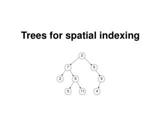
Trees for spatial indexing Part 2 : SAMs
SAMs R-Tree R*-Tree X TV
Answering question • The Kd-Trie, is similar to kd-tree. In the article it was used for kd-tree. • The split-axis isn’t in the middle, but is choosen is the median point. • Because, we work with points, we have no problem is separating the elements.
UB-Tree range queries • Algorithm is : • Find all region who intersects q • IF this region is a page, all objects that intersects q is in the answer. • After that we search for the last subcube in this region and we search the brother, and if it intersects q we make the same loop on it. • After that we look the father of B and search again.
R-Tree • Special B+-Tree for spatial indexing. • The performance of the R*-Tree is decreasing with the dimensionality. • R-tree access method is prohibitively slow for dimensions higher than 5.
Problems of (R-Tree based) Index Structures • Because it has been shown that with the increasing of the dimensionality we have also more overlap. • Overlap is intuitively when for some point queries, we have multiple paths to search.
Definition of overlap • Intuitively, overlap is the pourcentage of the volume that is covered by more than one directory hyperrectangle. • This intuitive definition of overlap is directly correlated to the query performance. • Because it implies multiple paths.
Definition of the overlap (2) • Overlap = ||( Ui,j, i≠j Ri∩ Rj )|| / ||( Ui Ri )|| • We add all the intersection of the MBR in volume and we divide it by the union of all the MBR in volume. • But overlap in highly populated areas is much more critical than overlap in low population. • WeightedOverlap = |{ p|p Ui,j,i≠j Ri∩ Rj )}| / |(p|p Ui Ri )|
1 1 Overlap = (¼)/(2) = 1/8 = 12,5 % WeightedOverlap = (2)/(6) = 1/3 = 33 %
Overlap / WeightedOverlap • Depending the kind of data the the measurement can be different. • If we have uniformed distributed data points, we can use the overlap measure • In the case of real data, when can have clustering, so the weightedOverlap is more accurate.
X-Tree • Avoid overlap in the directory. • X-Tree hybrid of a linear array-like and a hierarchical R-Tree-like directory. • In low dimensions the most efficient organization of the directory is hierarchical organization. • For high dimensionality a linear organization is more efficient.
X-Tree • In the X-Tree we have 3 types of nodes : data nodes,normal directory, and supernodes. • The supernodes avoid splits in directory, so it’s more faster to search. • Not the same as R*-Tree with larger blocks, because it creates larger blocks only if necessary.
X-Tree Supernode Normal directory Data nodes
Creation of supernodes • They are only created if there is no other possibility to avoid overlap during insertion.
TV-Tree (Telescopic-Vector tree) • The basis of the tv-tree is to use dynamically contracting and extending feature vectors. ( Like in classification )
TV-Tree • A m-contraction of x, is a sequence of • Amx where Am is a contraction matrix. • A natural Am is • ( 1 0 … 0 )( 0 1 0 … 0 )( …. )( 0 …. 0 1)
Multiple shapes • We can use for example a sphere, because it’s only a center and a radius r. Represents the set of points with euclidean distance ≤ r. • ~the euclidean distance is a special case of the Lp metrics with p=2. • For L1 metric (manhattan distance) it defines a diamond shape. • The TV-tree is working with any Lp-sphere.
Tv-Tree principle • So the TV treats the attributs asymmetrically favoring the first few features over the rest. • TV-Tree can use any type of MBR (minimum bounding region), rectangle,cube,sphere etc. • TV-Tree can use any Lp-Sphere
TV-Tree node structure • Each node is represents the MBR of all it’s descendents ( say an Lp-sphere ). • Each region is represented by a center which is a telescopic-vector and a radius. • So we talk about TMBR.
TMBR Act. Dim : y Act. Dim : x,z Act. Dim : z Act. Dim : x,y Act. Dim : x
What is the best number of active dimensions ? • They find out that the best number of active dimensions was two
TV-Tree conclusion • We accept overlap, so also multiple path to search. • Branch choosen for new point is done with the following criteria :