Download
1 / 20
200 likes | 377 Views
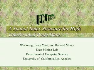
PK tree. A Spatial Index Structure for High Dimensional Point Data. Wei Wang, Jiong Yang, and Richard Muntz Data Mining Lab Department of Computer Science University of California, Los Angeles. Outline. Introduction Structure of PK-tree Operations on PK-tree Performance Conclusions.

E N D
PK tree A Spatial Index Structure for High Dimensional Point Data Wei Wang, Jiong Yang, and Richard Muntz Data Mining Lab Department of Computer Science University of California, Los Angeles
Outline • Introduction • Structure of PK-tree • Operations on PK-tree • Performance • Conclusions
Introduction • Dynamic spatial index method has been an active research area. • index structure based on spatial decomposition • PR-Quad tree, K-D tree, K-D-B tree, ... • No overlapping among sibling nodes • How to achieve high disk page utilization for large dimensionality with skewed data distributions remains a challenge. • R-tree family of index structure • R*-tree, SR-tree, X-tree, ... • Increasing of overlapping among sibling nodes along with increasing dimensionality degrades performance severely.
Introduction • PK-tree • Spatial decomposition • no overlapping among sibling nodes • Bound on height • Bounds on number of children • Uniqueness for any data set • independent of order of insertion and deletion • Solid theoretical foundation • Fast retrieval and updates
. . . . . . . . . ith level . . . . . . . . . (i+1)th level . . . dim 2 . . . dim 1 Structure of PK-tree • Recursively rectilinear dividing space Set notation (e.g., , , , , , , ) is used to express relationships among cells.
Space is recursively divided until a level LD such that each cell contains at most one point. . . . . . . . . . . . . . . . . . . . . . . . . . . . . . . . . . . . . . . . . . . . . . . . . . . . . . . . . . . . . . . . . . . . . . . . . . . . . . . . . . . . . . . . . . . . . . . . . Level 0 Level 1 Level 2 Level 3 Structure of PK-tree
Point cell: a non-empty cell at level LD A cell C is K-instantiable iff C is a point cell, or there does not exist (K-1) or less K-instantiable sub-cells C1, …, CK-1 C, such that d D (d C d i=0K-1Ci). . . . . . . . . . . . . . . . . . . . . . . . . . . . . . . . . . . . . K = 3 . . . . . . . . . . . . Level 3 (LD) Level 2 Level 1 . . . . . . . . . . . . . . . . . . . . . . . . Structure of PK-tree
. . . . . . . . . . . . . . . . . . . . 1 . . . 1 1 . . . B D 2 . 2 2 . U R 3 . . . 3 3 . . . 4 . 4 4 . 5 . . . 5 5 . . . K K 6 . . . 6 6 . . . 7 7 7 M N M N 8 8 8 a b c d e f g h a b c d e f g h a b . c d . e . f g . h . . . . . . Level 3 (LD) Level 2 Level 1 . . . root . B D M N K . . . . U R a2 d1 c2 d2 b4 c3 e1 e2 f3 g1 h1 g2 h2 g3 a7 b7 . b8 . d7 . c8 d8 e5 f5 f6 g5 . . . Structure of PK-tree Example of a PK-tree of rank 3
Structure of PK-tree • Given a finite set of points D over index space C0 and dividing ration R, a PK-tree of rank K (K>1) is defined as follows. • The cell at level 0 (C0) is always instantiated and serves as therootof the PK-tree. • Every node else (except the root) in the PK-tree is mapped one-to-one to a K-instantiable cell. • For any two nodes C1 and C2 in the PK-tree, C1 is a child of C2 (or C2 is the parent of C1) iff • C1 is a proper sub-cell of C2, i.e., C1 C2, and • there does not exist C3 in the PK-tree such that C1 C3 and C3 C2. • Properties: existence and uniqueness, bounds on node outdegree, bounded storage space, bounds on expected height, no overlapping among sibling nodes, and so on.
root (N points) ... at least K-1 Ci H ... at least K-1 Ci+1 P(d Ci+1 | d Ci) < 1 ... at least K-1 ... at least K-1 leaf longest path Properties of PK-tree Expected Height of a PK-tree
... Ac ... Ci+1 ... ... Ci A Properties of PK-tree • M-Level Clustering Spatial Distribution • 0-level: uniform distribution over C0 P(d Ci+1 | d Ci) = 1/r • 1-level: Let A C0 be some subset of C0 and Ac = C0 - A. Distributions for points in A and Ac are 0-level clustering spatial distribution.
Operations on PK-tree • Pagination of the PK-tree • Pick the parameter K and the number of dimensions to split at each level such that the maximum size node is close to a page size. • Allocate one node to a page. • Space utilization can be guaranteed to be at least 50% and is much more than 50% in experiments. • Insertion • First follow the path from the root to locate all (potential) ancestors of the inserted leaf cell. • Then from the leaf level back to the root along the same path to make all necessary changes (e.g., instantiate or de-instantiate cells). • Search • K Nearest Neighbor Query • Range Query
Performance • Setup: Sparc 10 workstation (SunOS 5.5) with 208 MB main memory and a local disk with 9GB capacity • Synthetic Data Sets (each contains 100,000 points) • u: uniform distribution • c1, c2: 20% of data are uniformly distributed and 80% of data are distributed in disjoint clusters • Height of generated trees
Performance • Size of index in MB with 100,000 points
Performance • Range query on uniform data distribution
Performance • Range query on clustered data distribution
Performance • KNN query on uniform data distribution
Performance • KNN query on clustered data distribution
Performance • Real data set: NASA Sky Telescope Data • 200,000 two-dimensional points (they are the coordinates of crater locations on the surface of Mars)
Conclusions • PK-tree: employing spatial decomposition to ensure no overlapping among sibling nodes but avoiding large number of nodes usually resulting from a skewed spatial distribution of objects. • The total number of nodes in a PK-tree is O(N) and the expected height of a PK-tree is O(logN) under some general conditions. • Other properties: uniqueness, bounds on number of children. • Empirical studies shown that the PK-tree outperforms SR-tree and X-tree by a wide margin.