Download
1 / 96
1.05k likes | 1.44k Views
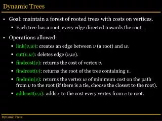
Dynamic Trees. Goal: maintain a forest of rooted trees with costs on vertices. Each tree has a root, every edge directed towards the root. Operations allowed: link( v , w ) : creates an edge between v (a root) and w . cut( v , w ) : deletes edge ( v , w ).

E N D
Dynamic Trees • Goal: maintain a forest of rooted trees with costs on vertices. • Each tree has a root, every edge directed towards the root. • Operations allowed: • link(v,w): creates an edge between v (a root) and w. • cut(v,w): deletes edge (v,w). • findcost(v): returns the cost of vertex v. • findroot(v): returns the root of the tree containing v. • findmin(v): returns the vertex w of minimum cost on the path from v to the root (if there is a tie, choose the closest to the root). • addcost(v,x): adds x to the cost every vertex from v to root. Dynamic Trees
Dynamic Trees • An example (two trees): a 3 b c 6 2 1 d j 1 7 e 4 f g 3 h 9 i 4 l 8 6 k 7 2 m n o 4 p 6 q 1 s 2 r 8 t 6 u 4 Dynamic Trees
Dynamic Trees a a 3 3 b c 6 2 b c 6 2 1 d 1 d j j 1 7 link(q,e) 1 7 e 4 e 4 f g 3 h 9 i 4 f g 3 h 9 i 4 l 8 6 q l 8 6 k 7 2 1 k 7 2 m n m n s 2 r 8 o 4 p 6 o 4 p 6 q 1 t 6 u 4 s 2 r 8 t 6 u 4 Dynamic Trees
Dynamic Trees a a 3 3 b c 6 2 b c 6 2 1 d 1 d j j 1 7 cut(q) 1 7 e 4 e 4 f g 3 h 9 i 4 f g 3 h 9 i 4 l 8 6 q l 8 6 k 7 2 1 k 7 2 m n m n s 2 r 8 o 4 p 6 o 4 p 6 q 1 t 6 u 4 s 2 r 8 t 6 u 4 Dynamic Trees
Dynamic Trees • findmin(s) = b • findroot(s) = a • findcost(s) = 2 • addcost(s,3) a 3 b c 6 2 1 d j 1 7 e 4 f g 3 h 9 i 4 q l 8 6 1 k 7 2 m n s 2 r 8 o 4 p 6 t 6 u 4 a 6 b c 6 2 4 d j 1 7 e 7 f g 3 h 9 i 4 q l 8 6 4 k 7 2 m n s 5 r 8 o 4 p 6 t 6 u 4 Dynamic Trees
Obvious Implementation • A node represents each vertex; • Each node x points to its parent p(x): • cut, split, findcost: constant time. • findroot, findmin, addcost: linear time on the size of the path. • Acceptable if paths are small, but O(n) in the worst case. • Cleverer data structures achieve O(log n) for all operations. Dynamic Trees
Simple Paths • We start with a simpler problem: • Maintain set of paths subject to: • split: cuts a path in two; • concatenate: links endpoints of two paths, creating a new path. • Operations allowed: • findcost(v): returns the cost of vertex v; • addcost(v,x): adds x to the cost of vertices in path containing v; • findmin(v): returns minimum-cost vertex path containing v. v1 v2 v3 v4 v5 v6 v7 Dynamic Trees
Simple Paths as Lists • Natural representation: doubly linked list. • Constant time for findcost. • Constant time for concatenate and split if endpoints given, linear time otherwise. • Linear time for findminand addcost. • Can we do it O(log n) time? costs: 6 2 3 4 7 9 3 v1 v2 v3 v4 v5 v6 v7 Dynamic Trees
Simple Paths as Binary Trees • Alternative representation: balanced binary trees. • Leaves: vertices in symmetric order. • Internal nodes: subpaths between extreme descendants. (v1,v7) (v4,v7) (v1,v3) (v4,v6) (v1,v2) (v5,v6) v1 v2 v3 v4 v5 v6 v7 Dynamic Trees
Simple Paths as Binary Trees • Compact alternative: • Each internal node represents both a vertex and a subpath: • subpath from leftmost to rightmost descendant. v6 v2 v7 v1 v4 v3 v5 v1 v2 v3 v4 v5 v6 v7 Dynamic Trees
Simple Paths: Maintaining Costs • Keeping costs: • First idea: store cost(x) directly on each vertex; • Problem: addcost takes linear time (must update all vertices). actual costs 9 v6 2 v2 3 v7 6 v1 4 v4 3 v3 7 v5 costs: 6 2 3 4 7 9 3 v1 v2 v3 v4 v5 v6 v7 Dynamic Trees
Simple Paths: Maintaining Costs • Better approach: store cost(x) instead: • Root: cost(x) = cost(x) • Other nodes: cost(x) = cost(x) –cost(p(x)) actual costs 9 v6 difference form 9 v6 2 v2 3 v7 -7 v2 -6 v7 6 v1 4 v4 4 v1 2 v4 3 v3 7 v5 -1 v3 3 v5 costs: 6 2 3 4 7 9 3 v1 v2 v3 v4 v5 v6 v7 Dynamic Trees
Simple Paths: Maintaining Costs • Costs: • addcost: constant time (just add to root) • Finding cost(x)is slightly harder: O(depth(x)). actual costs 9 v6 difference form 9 v6 2 v2 3 v7 -7 v2 -6 v7 6 v1 4 v4 4 v1 2 v4 3 v3 7 v5 -1 v3 3 v5 costs: 6 2 3 4 7 9 3 v1 v2 v3 v4 v5 v6 v7 Dynamic Trees
Simple Paths: Finding Minima • Still have to implement findmin: • Store mincost(x), theminimum cost on subpath with root x. • findmin runs in O(log n) time, but addcost is linear. actual costs 9 v6 mincost 2 v6 2 v2 3 v7 2 v2 3 v7 6 v1 4 v4 6 v1 3 v4 3 v3 7 v5 3 v3 7 v5 costs: 6 2 3 4 7 9 3 v1 v2 v3 v4 v5 v6 v7 Dynamic Trees
Simple Paths: Finding Minima • Store min(x) = cost(x)–mincost(x) instead. • findmin still runs in O(log n) time, addcost now constant. actual costs 9 v6 mincost 2 v6 min 7 v6 2 v2 3 v7 2 v2 3 v7 0 v2 0 v7 6 v1 4 v4 6 v1 3 v4 0 v1 1 v4 3 v3 7 v5 3 v3 7 v5 0 v3 0 v5 costs: 6 2 3 4 7 9 3 v1 v2 v3 v4 v5 v6 v7 Dynamic Trees
Simple Paths: Data Fields • Final version: • Stores min(x) and cost(x) for every vertex actual costs 9 v6 (cost, min) (9, 7) v6 2 v2 3 v7 (-7,0) v2 (-6,0) v7 6 v1 4 v4 (4,0) v1 (2,0) v4 3 v3 7 v5 (1,0) v3 (3,0) v5 costs: 6 2 3 4 7 9 3 v1 v2 v3 v4 v5 v6 v7 Dynamic Trees
Simple Paths: Structural Changes • Concatenating and splitting paths: • Join or split the corresponding binary trees; • Time proportional to tree height. • For balanced trees, this is O(log n). • Rotations must be supported in constant time. • We must be able to update min and cost. Dynamic Trees
Simple Paths: Structural Changes • Restructuring primitive: rotation. • Fields are updated as follows (for left and right rotations): • cost’(v) = cost(v) + cost(w) • cost’(w) = –cost(v) • cost’(b) = cost(v) + cost(b) • min’(w) = max{0, min(b) – cost’(b), min(c) – cost(c)} • min’(v) = max{0, min(a) – cost(a), min’(w) – cost’(w)} w v rotate(v) v c a w a b b c Dynamic Trees
Splaying • Simpler alternative to balanced binary trees: splaying. • Does not guarantee that trees are balanced in the worst case. • Guarantees O(log n) access in the amortized sense. • Makes the data structure much simpler to implement. • Basic characteristics: • Does not require any balancing information; • On an access to v, splay on v: • Moves v to the root; • Roughly halves the depth of other nodes in the access path. • Based entirely on rotations. • Other operations (insert, delete, join, split) use splay. Dynamic Trees
Splaying • Three restructuring operations: z x y y z D zigzag(x) A B C D x A z x B C y y D A zigzig(x) x C z B A B C D y x zig(x) x y C A A B B C (only happens if y is root) Dynamic Trees
An Example of Splaying h g I f H e A d G c B b C a D E F Dynamic Trees
An Example of Splaying h h g g I I f f H H e e A A d zigzig(a) d G G c a B B b b C F a c D E E F C D Dynamic Trees
An Example of Splaying h g I f H e A d G a B b F c E C D Dynamic Trees
An Example of Splaying h h g g I I f f H H a e A A d e zigzag(a) d G b a B F G B c b E F c C D E C D Dynamic Trees
An Example of Splaying h g I f H a A d e b B F G c E C D Dynamic Trees
An Example of Splaying h h g a I I f f H g a A A d e H d e zigzag(a) b B F G b B F G c E c E C D C D Dynamic Trees
An Example of Splaying h a I f g A d e H b B F G c E C D Dynamic Trees
An Example of Splaying a h f h a I d g f A I g b e B H A d e H c zig(a) E F G b B F G C D c E C D Dynamic Trees
An Example of Splaying a f h d g A I b e B H c E F G C D Dynamic Trees
An Example of Splaying • End result: h a g f h I f d g H A I e b e A B H d splay(a) c G E F G c B C D b C a D E F Dynamic Trees
Amortized Analysis • Bounds the running time of a sequence of operations. • Potential function maps each configuration to real number. • Amortized time to execute each operation: • ai = ti + i– i –1 • ai: amortized time to execute i-th operation; • ti: actual time to execute the operation; • i: potential after the i-th operation. • Total time for m operations: i=1..mti = i=1..m(ai+ i –1–i) = 0 –m + i=1..mai Dynamic Trees
Amortized Analysis of Splaying • Definitions: • s(x): size of node x (number of descendants, including x); • At most n, by definition. • r(x): rank of node x, defined as log s(x); • At most log n, by definition. • i: potential of the data structure (twice the sum of all ranks). • At most O(n log n), by definition. • Access Lemma [ST85]: The amortized time to splay a tree with root t at a node x is at most 6(r(t)–r(x)) + 1 = O(log(s(t)/s(x))). Dynamic Trees
Proof of Access Lemma • Access Lemma [ST85]: The amortized time to splay a tree with root t at a node x is at most 6(r(t)–r(x)) + 1 = O(log(s(t)/s(x))). • Proof idea: • ri(x) = rank of x after the i-th splay step; • ai = amortized cost of the i-th splay step; • ai 6(ri(x)–ri–1(x)) + 1 (for the zig step, if any) • ai 6(ri(x)–ri–1(x)) (for any zig-zig and zig-zag steps) • Total amortized time for all k steps: i=1..kai i=1..k-1 [6(ri(x)–ri–1(x))] + [6(rk(x)–rk–1(x)) + 1] = 6rk(x) – 6r0(x) + 1 Dynamic Trees
Proof of Access Lemma: Splaying Step • Zig-zig: Claim: a 6 (r’(x) – r(x)) t + ’– 6 (r’(x) – r(x)) 2 + 2(r’(x)+r’(y)+r’(z))– 2(r(x)+r(y)+r(z)) 6 (r’(x) – r(x)) 1+ r’(x) + r’(y) + r’(z) – r(x) – r(y) – r(z) 3 (r’(x) – r(x)) 1 + r’(y) + r’(z) – r(x) – r(y) 3 (r’(x) – r(x)) since r’(x) = r(z) 1 + r’(y) + r’(z) – 2r(x) 3 (r’(x) – r(x)) since r(y) r(x) 1 + r’(x) + r’(z) – 2r(x) 3 (r’(x) – r(x)) since r’(x) r’(y) (r(x) – r’(x)) + (r’(z) – r’(x)) –1 rearranging log(s(x)/s’(x)) + log(s’(z)/s’(x)) –1 definition of rank TRUE because s(x)+s’(z)<s’(x): both ratios are smaller than 1, at least one is at most 1/2. z x y y D A zigzig(x) x C z B A B C D Dynamic Trees
Proof of Access Lemma: Splaying Step • Zig-zag: Claim: a 4(r’(x) – r(x)) t + ’– 4(r’(x) – r(x)) 2 + (2r’(x)+2r’(y)+2r’(z)) – (2r(x)+2r(y)+2r(z))4(r’(x) – r(x)) 2 + 2r’(y) + 2r’(z) – 2r(x) – 2r(y)4(r’(x) – r(x)), since r’(x) = r(z) 2 + 2r’(y) + 2r’(z) – 4r(x)4(r’(x) – r(x)), since r(y) r(x) (r’(y) – r’(x)) + (r’(z) –r’(x)) –1, rearranging log(s’(y)/s’(x)) + log(s’(z)/s’(x)) –1 definition of rank TRUE because s’(y)+s’(z)<s’(x): both ratios are smaller than 1, at least one is at most 1/2. z x y y z D zigzag(x) A B C D x A B C Dynamic Trees
Proof of Access Lemma: Splaying Step • Zig: Claim: a 1 + 6(r’(x) – r(x)) t + ’– 1 + 6 (r’(x) – r(x)) 1 + (2r’(x)+2r’(y)) – (2r(x)+2r(y))1 + 6(r’(x) – r(x)) 1 + 2 (r’(x) – r(x)) 1 +6(r’(x) – r(x)), since r(y) r’(y) TRUE because r’(x) r(x). y x zig(x) x y C A A B B C (only happens if y is root) Dynamic Trees
Splaying • To sum up: • No rotation: a = 1 • Zig: a 6(r’(x) – r(x)) + 1 • Zig-zig: a 6(r’(x) – r(x)) • Zig-zag: a 4(r’(x) – r(x)) • Total amortized time at most 6 (r(t) – r(x)) + 1 = O(log n) • Since accesses bring the relevant element to the root, other operations (insert, delete, join, split) become trivial. Dynamic Trees
Dynamic Trees • We know how to deal with isolated paths. • How to deal with paths within a tree? Dynamic Trees
Dynamic Trees • Main idea: partition the vertices in a tree into disjoint solid paths connected by dashededges. Dynamic Trees
Dynamic Trees • Main idea: partition the vertices in a tree into disjoint solid paths connected by dashededges. Dynamic Trees
Dynamic Trees • A vertex v is exposed if: • There is a solid path from v to the root; • No solid edge enters v. Dynamic Trees
Dynamic Trees • A vertex v is exposed if: • There is a solid path from v to the root; • No solid edge enters v. • It is unique. v Dynamic Trees
Dynamic Trees • Solid paths: • Represented as binary trees (as seen before). • Parent pointer of root is the outgoing dashed edge. • Hierarchy of solid binary trees linked by dashed edges: “virtual tree”. • “Isolated path” operations handle the exposed path. • The solid path entering the root. • Dashed pointers go up, so the solid path does not “know” it has dashed children. • If a different path is needed: • expose(v): make entire path from v to the root solid. Dynamic Trees
Virtual Tree: An Example a b f c b d l f c e g q i a i h p k j l j h m k o p q n m e r s n o d t r t g v u s v w u w virtual tree actual tree Dynamic Trees
Dynamic Trees • Example: expose(v) v Dynamic Trees
Dynamic Trees • Example: expose(v) • Take all edges in the path to the root, … v Dynamic Trees
Dynamic Trees • Example: expose(v) • …, make them solid, … v Dynamic Trees
Dynamic Trees • Example: expose(v) • …make sure there is no other solid edge incident into the path. • Uses splice operation. v Dynamic Trees
Exposing a Vertex • expose(x): makes the path from x to the root solid. • Implemented in three steps: • Splay within each solid tree in the path from x to root. • Splice each dashed edge from x to the root. • splice makes a dashed become the left solid child; • If there is an original left solid child, it becomes dashed. • Splay on x, which will become the root. Dynamic Trees
Exposing a Vertex: An Example • expose(a) l k a k k l k pass 1 f f pass 2 l pass 3 j j b l b b j i i f i g g e e a h a e i h c h g c j c d d g d f h e d c b a (virtual trees) Dynamic Trees