Download
1 / 26

E N D
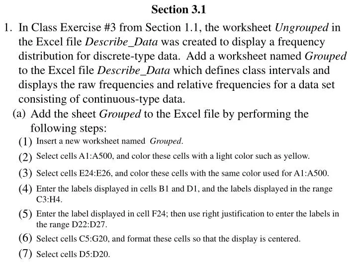
Section 3.1 1. (a) In Class Exercise #3 from Section 1.1, the worksheet Ungrouped in the Excel file Describe_Data was created to display a frequency distribution for discrete-type data. Add a worksheet named Grouped to the Excel file Describe_Data which defines class intervals and displays the raw frequencies and relative frequencies for a data set consisting of continuous-type data. Add the sheet Grouped to the Excel file by performing the following steps: (1) (2) (3) (4) Insert a new worksheet named Grouped. Select cells A1:A500, and color these cells with a light color such as yellow. Select cells E24:E26, and color these cells with the same color used for A1:A500. Enter the labels displayed in cells B1 and D1, and the labels displayed in the range C3:H4. (5) Enter the label displayed in cell F24; then use right justification to enter the labels in the range D22:D27. (6) (7) Select cells C5:G20, and format these cells so that the display is centered. Select cells D5:D20.
(8) From the main menu select the Formulas tab, select the option Name Manager, and click the New button in the dialog box which appears. (9) Type the new range name Limits (if it is not already displayed), and click the OK button to return to the Name Manager dialog box. (10) With the Name Manager dialog box still open, click the New button, type the new range name RawData (no spaces!), and click inside the Refers to slot.
(11) With the Refers to slot selected, highlight cells A1:A500, and click the OK button to return to the Name Manager dialog box. (12) With the Name Manager dialog box still open, click the New button, type the new range name Length, and click inside the Refers to slot. (13) With the Refers to slot selected, select cell E27, and click the OK button to return to the Name Manager dialog box. (14) With the Name Manager dialog box still open, click the New button, type the new range name NumClass, and click inside the Refers to slot. (15) With the Refers to slot selected, select cell E24, click the OK button to return to the Name Manager dialog box, and click the Close button to close the dialog box. (16) (17) (18) (19) Enter the following formula in cell C5: =IF(ISNUMBER(Length),E25,"-") Enter the following formula in cell D5: =IF(C5="-","-",C5+Length) Copy the formula in D5 down to cells D6:D20. Enter the following formula in cell C6: =IF(AND(ISNUMBER(Length),NumClass>=2),D5,"-")
(20) (21) Copy the formula in C6 down to cells C7:C20. Edit cell C7 to change >=2 to >=3, edit cell C8 to change >=2 to >=4, edit cell C9 to change >=2 to >=5, etc. (You should finish by editing C20 to change >=2 to >=16.) (22) Select cells E5:E20. (23) Type the following formula (but do not press the {Enter} key!): =IF(Limits="-","-",FREQUENCY(RawData,Limits)) (24) (25) (26) (27) (28) (29) While holding down the {Shift} and {Ctrl} keys together, press {Enter}. Enter the following formula in cell F5: =IF(Limits="-","-",E5/COUNT(RawData)) Copy the formula in F5 down to cells F6:F20. Enter the following formula in cell G5: =IF(Limits="-","-",F5/Length) Copy the formula in G5 down to cells G6:G20. Enter the following formula in cell E22: =IF(COUNT(RawData)>0,MIN(RawData),"") (30) Enter the following formula in cell E23: =IF(COUNT(RawData)>0,MAX(RawData),"") (31) Enter the following formula in cell E27: =IF(AND(COUNT(RawData)>0,ISNUMBER(NumClass), ISNUMBER(E25),ISNUMBER(E26)),(E26-E25)/NumClass,"")
(32) Enter the following formula in cell H5: =IF(Limits="-","-",(C5+D5)/2) (33) Copy the formula in H5 down to cells H6:H20. (34) Save the file as Describe_Data (in your personal folder on the college network). (b) In Class Exercise #2 from Section 2.1, the data from Text Exercise 2.1-4 was used to construct a frequency distribution for the individual digits was obtained using worksheet Ungrouped. Now use the worksheet Grouped to obtain a frequency distribution for the three-digit numbers, with 10 classes: from 000 to 100, from 101 to 200, from 201 to 300, etc. (available in Excel file Data_for_Students). (c) Use the worksheet Grouped to obtain Table 3.1-2 of the textbook from the data of Table 3.1-1 for Example 3.1-1 (available in Excel file Data_for_Students).
2. (a) In Class Exercise #1, a sheet named Grouped was added to the Excel file Describe_Data which defines class intervals and displays the raw frequencies and relative frequencies for a data set consisting of continuous-type data. Modify the sheet Grouped so that the mean, variance, and standard deviation are displayed when calculated from the raw data and also when calculated from the frequency distribution. Modify the sheet Grouped by performing the following steps: (1) In the worksheet named Grouped, add the labels displayed in cells I4 and J4. (2) Add the labels displayed in cells C30 and I30; then format these cells so that the display is underlined. (3) Use right justification to enter the labels in the range D31:D34 and the labels in the range J31:J34.
(4) (5) (6) Select I5:J20, and format these cells so that the display is centered. Select cell K31. From the main menu select the Formulas tab, select the option Name Manager, and click the New button in the dialog box which appears. (7) Type the new range name Mean, and click the OK button to return to the Name Manager dialog box. (8) With the Name Manager dialog box still open, click the New button, type the new range name Marks, and click inside the Refers to slot. (9) With the Refers to slot selected, highlight cells H5:H20, click the OK button to return to the Name Manager dialog box, and click the Close button to close the dialog box.
(10) (11) (12) (13) Enter the following formula in cell I5: =IF(Limits="-","-",E5*Marks) Enter the following formula in cell J5: =IF(Limits="-","-",E5*(Marks-Mean)^2) Copy the formulas in I5:J5 down to cells I6:J20. Format the cells E31:E34 and the cells K31:K34 so that the display is centered. (14) Enter the following formulas respectively in cells E31:E34 : =IF(C5="-","-",AVERAGE(RawData)) =IF(C5="-","-",VAR(RawData)) =IF(C5="-","-",STDEV(RawData)) =COUNT(RawData) (15) Enter the following formulas respectively in cells K31:K34 : =IF(C5="-","-",SUM(I5:I20)/SUM(E5:E20)) =IF(C5="-","-",SUM(J5:J20)/(SUM(E5:E20)-1)) =IF(C5="-","-",SQRT(K32)) =SUM(E5:E20) (16) Save the file as Describe_Data (in your personal folder on the college network).
(b) Use the worksheet Grouped in the Excel file Describe_Data to obtain Table 3.1-2 of the textbook from the data of Table 3.1-1 for Example 3.1-1 (available in Excel file Data_for_Students). Then, verify that the mean and variance calculated from the grouped data are respectively 23.51 and 2.5671, and compare these to the mean and variance calculated from the raw data.
Section 3.2 1. (a) The lifetimes in hours for a sample of 30 Econo brand light bulbs were recorded as follows: 1078 879 890 1001 1027 990 888 1224 1008 1017 996 895 997 992 999 882 885 897 1004 1051 1012 994 1199 1147 889 893 881 892 1032 1101 Construct a stem-and-leaf display. 8 79, 90, 88, 95, 82, 85, 97, 89, 93, 81, 92 9 90, 96, 97, 92, 99, 94 10 78, 01, 27, 08, 17, 04, 51, 12, 32 11 99, 47, 01 12 24 8 79, 81, 82, 85, 88, 89, 90, 92, 93, 95, 97 9 90, 92, 94, 96, 97, 99 10 01, 04, 08, 12, 17, 27, 32, 51, 78 11 01, 47, 99 12 24
(b) Find the five-number summary, the 10th percentile, and the 90th percentile. Use both the textbook formula and the Excel formula. sample of size n: x1 , x2 , …, xn sample order statistics: y1 , y2 , …, yn Textbook formula for the (100p)th percentile in a sample of size n: Excel formula for the (100p)th percentile in a sample of size n: yr + (a/b)(yr + 1–yr) where r is the integer part of (n + 1)p and a/b is the proper fraction part of (n + 1)p yr + 1 + (a/b)(yr + 2–yr + 1) where r is the integer part of (n 1)p and a/b is the proper fraction part of (n 1)p
(b) Find the five-number summary, the 10th percentile, and the 90th percentile. Use both the textbook formula and the Excel formula. 8 79, 81, 82, 85, 88, 89, 90, 92, 93, 95, 97 9 90, 92, 94, 96, 97, 99 10 01, 04, 08, 12, 17, 27, 32, 51, 78 11 01, 47, 99 12 24 The five-number summary according to the textbook is 879 996.5 1224 The five-number summary according to Excel is 879 996.5 1224 n = 30 p = 0.5 With the textbook: With the Excel: (n+ 1)p = 15.5 50th percentile = y15 + (0.5)(y16–y15) (n– 1)p = 14.5 50th percentile = y15 + (0.5)(y16–y15)
(b) Find the five-number summary, the 10th percentile, and the 90th percentile. Use both the textbook formula and the Excel formula. 8 79, 81, 82, 85, 88, 89, 90, 92, 93, 95, 97 9 90, 92, 94, 96, 97, 99 10 01, 04, 08, 12, 17, 27, 32, 51, 78 11 01, 47, 99 12 24 The five-number summary according to the textbook is 879 891.5 996.5 1224 The five-number summary according to Excel is 879 892.25 996.5 1224 n = 30 p = 0.25 With the textbook: With the Excel: (n+ 1)p = 7.75 25th percentile = y7 + (0.75)(y8–y7) (n– 1)p = 7.25 25th percentile = y8 + (0.25)(y9–y8)
(b) Find the five-number summary, the 10th percentile, and the 90th percentile. Use both the textbook formula and the Excel formula. 8 79, 81, 82, 85, 88, 89, 90, 92, 93, 95, 97 9 90, 92, 94, 96, 97, 99 10 01, 04, 08, 12, 17, 27, 32, 51, 78 11 01, 47, 99 12 24 The five-number summary according to the textbook is 879 891.5 996.5 1028.25 1224 The five-number summary according to Excel is 879 892.25 996.5 1024.5 1224 n = 30 p = 0.75 With the textbook: With the Excel: (n+ 1)p = 23.25 75th percentile = y23 + (0.25)(y24–y23) (n– 1)p = 21.75 75th percentile = y22 + (0.75)(y23–y22)
(b) Find the five-number summary, the 10th percentile, and the 90th percentile. Use both the textbook formula and the Excel formula. 8 79, 81, 82, 85, 88, 89, 90, 92, 93, 95, 97 9 90, 92, 94, 96, 97, 99 10 01, 04, 08, 12, 17, 27, 32, 51, 78 11 01, 47, 99 12 24 The 10th percentile according to the textbook is 882.3 hours. The 10th percentile according to Excel is 884.7 hours. n = 30 p = 0.10 With the textbook: With the Excel: (n+ 1)p = 3.1 10th percentile = y3 + (0.1)(y4–y3) (n– 1)p = 2.9 10th percentile = y3 + (0.9)(y4–y3)
(b) Find the five-number summary, the 10th percentile, and the 90th percentile. Use both the textbook formula and the Excel formula. 8 79, 81, 82, 85, 88, 89, 90, 92, 93, 95, 97 9 90, 92, 94, 96, 97, 99 10 01, 04, 08, 12, 17, 27, 32, 51, 78 11 01, 47, 99 12 24 The 90th percentile according to the textbook is 1142.4 hours. The 90th percentile according to Excel is 1105.6 hours. n = 30 p = 0.90 With the textbook: With the Excel: (n+ 1)p = 27.9 90th percentile = y27 + (0.9)(y28–y27) (n– 1)p = 26.1 90th percentile = y27 + (0.1)(y28–y27)
(c) Construct a box-and-whisker plot (box plot), using the five-number summary calculated from the textbook formula in part (b). The five-number summary according to the textbook is 879 891.5 996.5 1028.25 1224 850 900 950 1000 1050 1100 1150 1200 1250 1300 Bulb Lifetime (Hours)
2. (a) In a sample of 25 male grackles, each at least one year old, the wing chords were measured in centimeters and recorded as follows: 14.1 14.0 13.9 14.4 13.0 13.6 14.3 13.6 13.8 14.1 13.7 14.3 14.2 13.4 14.1 13.5 14.8 14.4 13.8 14.0 13.5 14.5 13.5 13.8 14.4 Construct a stem-and-leaf display with stems 13.-, 13.t, 13.f, 13.s, 13.*, 14.-, etc. 13.- 0 13.- 0 13.t 13.t 13.f 4 5 5 5 13.f 4 5 5 5 13.s 6 6 7 13.s 6 6 7 13.* 9 8 8 8 13.* 8 8 8 9 14.- 1 0 1 1 0 14.- 0 0 1 1 1 14.t 3 3 2 14.t 2 3 3 14.f 4 4 5 4 14.f 4 4 4 5 14.s 14.s 14.* 8 14.* 8
(b) Find the five-number summary, the 15th percentile, and the 85th percentile. Use both the textbook formula and the Excel formula.
(c) Construct a box-and-whisker plot (box plot), using the five-number summary calculated from the textbook formula in part (b).
3. (a) In Class Exercise #9 from Section 2.3, a sheet named Summary Stats was added to the Excel file Describe_Data which displays the mean, variance, and standard deviation for a sample. Modify the sheet Summary Stats so that the five-number summary, the IQR (interquartile range), and selected percentiles are also displayed. Modify the sheet Summary Stats by performing the following steps: (1) In the worksheet named Summary Stats, add the labels displayed in cells E7:E13, and right justify these labels. (2) Add the labels displayed in cells E15 and F16. (3) Color the cell E16 with a light color such as yellow. (4) Format the cell E17 so that the display is right justified.
(5) Enter the following formula in cell E17: =IF(AND(E16>0,E16<100),"The "&E16&"th percentile is","") (6) Enter the following formula in cell F17: =IF(AND(E16>0,E16<100),PERCENTILE(Sample,E16/100),"") (7) Enter the following formulas respectively in cells F7:F13: =IF(COUNT(Sample)>0,MIN(Sample),"-") =IF(COUNT(Sample)>0,QUARTILE(Sample,1),"-") =IF(COUNT(Sample)>0,MEDIAN(Sample),"-") =IF(COUNT(Sample)>0,QUARTILE(Sample,3),"-") =IF(COUNT(Sample)>0,MAX(Sample),"-") =IF(COUNT(Sample)>0,F10-F8,"-") =IF(COUNT(Sample)>0,F11-F7,"-") (8) Enter the following formula in cell H12: =IF(COUNT(Sample)>0,"The data contains","") (9) Enter the following formula in cell H13: =IF(COUNT(Sample)>0,IF(OR(F11-F10>1.5*F12,F8-F7>1.5*F12), "at least one potential outlier","no potential outliers"),"") (10) Save the file as Describe_Data (in your personal folder on the college network).
(b) For the data of Class Exercise #1 (available in Excel file Data_for_Students), use the worksheet Summary Stats in the Excel file Describe_Data to obtain the following: the sample mean, the sample variance, the sample standard deviation, the five-number summary, the IQR, the 10th percentile, the 90th percentile, and any potential outliers. Compare the five-number summary, the 10th percentile, and the 90th percentile displayed in Excel with the answers obtained by using the textbook formulas. (For convenience, the data in Class Exercise #1 is displayed here.) The lifetimes in hours for a sample of 30 Econo brand light bulbs were recorded as follows: 1078 879 890 1001 1027 990 888 1224 1008 1017 996 895 997 992 999 882 885 897 1004 1051 1012 994 1199 1147 889 893 881 892 1032 1101
(c) For the data of Class Exercise #2 (available in Excel file Data_for_Students), use the worksheet Summary Stats in the Excel file Describe_Data to obtain the following: the sample mean, the sample variance, the sample standard deviation, the five-number summary, the IQR, the 15th percentile, the 85th percentile, and any potential outliers. Compare the five-number summary, the 15th percentile, and the 85th percentile displayed in Excel with the answers obtained by using the textbook formulas. (For convenience, the data in Class Exercise #2 is displayed here.) In a sample of 25 male grackles, each at least one year old, the wing chords were measured in centimeters and recorded as follows: 14.1 14.0 13.9 14.4 13.0 13.6 14.3 13.6 13.8 14.1 13.7 14.3 14.2 13.4 14.1 13.5 14.8 14.4 13.8 14.0 13.5 14.5 13.5 13.8 14.4
Since the calculation of percentiles in Excel differs from the formulas in the textbook, add to the worksheet Summary Stats in the Excel file Describe_Data the following text box explaining the discrepancy: (d) Let n = 30. Suppose p = 0.01. With Excel: With the textbook: p(n– 1) = 0.29 1st percentile = y1 + (0.29)(y2–y1) p(n+ 1) = 0.31 1st percentile = y0 + (0.31)(y1–y0) What is this?!?
(e) For the data of Class Exercise #2 in Section 3.1, construct a box-and-whisker plot (box plot), which can be done easily by using the five-number summary from part (b).