Download
1 / 10

E N D
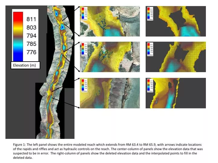
Elevation (m) Figure 1: The left panel shows the entire modeled reach which extends from RM 63.4 to RM 65.9, with arrows indicate locations of the rapids and riffles and act as hydraulic controls on the reach. The center-column of panels show the elevation data that was suspected to be in error. The right-column of panels show the deleted elevation data and the interpolated points to fill in the deleted data.
Figure 2: Measured water-surface profiles, modeled water-surface profiles, and stage-discharge relationships for all flows modeled.
Figure 3: The calibration curves of root-mean squared error as a function of the roughness coefficient (z-naught) for the three calibrated flow scenarios of 8,000, 16,000 and 43,100 ft3/s.
A B Figure 4: (A) The simulated Depth(m) at a flow of 8000 ft3/s for a portion of the entire reach modeled. (B) The difference in the simulated depth using a z0 roughness value of 0.07 and 0.10 The majority of the modeled reach shows that the sensitivity of depth to the calibrated roughness is less than 0.1 m. The mean depth at this flow is approximately 4 meters so the change in depth is 2.5 percent.
A B C Figure 5: (A) The simulated velocity (m/s) at a flow of 8000 ft3/s for a portion of the entire reach modeled. The difference in the simulated velocity using a z-naught roughness value of 0.07 and 0.10 are shown at two different scales: 0.0 – 0.04 m/s (values greater than 0.04 are plotted in red) in (B) and 0.05 – 0.50 m/s in (C). The riffles and rapids show the greatest sensitivity of velocity to the calibrated roughness values. The majority of the modeled reach shows that the sensitivity of velocity to the calibrated roughness is less than 0.05 m/s.
Figure 6: The simulated water-surface elevation (WSE) at a flow of 8000 ft3/s and the location of measured WSE (black squares). The blue arrows point to measured water-surface elevations that are lower than the elevation at that location. In regions where the geometry of the channel changes with the flow condition such as in the lateral-separation eddies the solution may not accurately represent the depth and velocity.
Figure 7: Example of the ASCII file output for each of the 5 modeled flows. x, y, and elevation are the three spatial locations of each node. IBC is a code for wet and dry nodes, -1 and 0, respectively. IBC can be used to mask the solution to show only those nodes that are wet. Depth and water-surface elevation are also given. Habitat suitability is 1 for all nodes with velocity less than 0.2 m/s and 0 for all others. Velocity magnitude and the x (VX_Velocity) and y (VY_Velocity) vector components, in geographical coordinates, is also given. The z (VZ_Velocity) vector component of velocity is always 0.
A B C D E F Figure 8: Red area’s indicate that the velocity is less than 0.2 m/s, for each of the six modeled flows including: 5000, 10000, 15000, 20000, 25000, and 45000 ft3/s (A-F respectively).
Figure 9: The Weighted Usable Area in meters-squared calculated for each of the six modeled flows. The calculation used a habitat suitability index of 1 for all computation nodes with a velocity less than 0.20 m/s and 0 for all nodes with a velocity greater than 0.20 m/s.
Figure 10: The persistence of flow area that experiences flow less than 0.20 m/s is plotted by summing the nodes for each of the six modeled discharges that have velocity less than 0.20 m/s, and normalize them by the number of flows. The resulting habitat persistence ranges from 0 to 1 with 1 representing area that fall within the specified habitat requirement across all flows.