Download
1 / 6
60 likes | 156 Views
ESM. Elevation: -5 m a.s.l . -35 m. -75 m. (Count/ 10 m). 10 8 6 4 2 0. 200 m. Fig. 1 Fracture density distributions at -5, -35, and -75 m a.s.l . constructed by SGS . ESM. 400 300 200 100 0. 4 3 2 1 0. (a). (b). Count . Semivariogram.

E N D
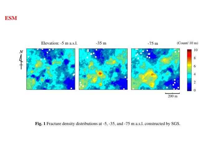
ESM Elevation: -5 m a.s.l. -35 m -75 m (Count/ 10 m) 10 8 6 4 2 0 200 m Fig. 1 Fracture density distributions at -5, -35, and -75 m a.s.l. constructed by SGS.
ESM 400 300 200 100 0 4 3 2 1 0 (a) (b) Count Semivariogram -6 -4 -2 0 2 4 6 0 100 200 300 400 Fracture apertures (cm) Distance (m) Fig. 2 a Histogram of fracture width data, and b omnidirectional experimental semivariogram and its approximation by a spherical model using the log-transformed data.
ESM 1.5 1 0.5 0 1.5 1 0.5 0 1.5 1 0.5 0 1.5 1 0.5 0 P1 P2 P3 P4 0 50 100 150 200 250 0 50 100 150 0 50 100 150 200 250 0 50 100 150 200 Semivariogram 1.5 1 0.5 0 1.5 1 0.5 0 2 1.5 1 0.5 0 P5 P6 P7 0 20 40 60 80 100 0 20 40 60 80 100 0 50 100 150 Distance (m) Fig. 3 Omnidirectional experimental semivariograms of the seven principal component values, P1 to P7, for the indicator sets of the fracture direction data.
1.170 1.169 1.168 1.167 1.166 1.165 1.164 ESM (%) N 3.5 3 2.5 2 1.5 1 0.5 0 Northing (×10 km) W E 0 2000 4000 6000 Count -5.88 -5.87 -5.86 -5.85 -5.84 -5.83 -5.82 -5.81 Easting (×10 km) Fig. 4 Fracture simulation result by GEOFRAC with the distributions of all the fractures including isolated fractures, strikes, and pole directions. Each fracture plane is expressed by a semitransparent plane colored randomly. The fracture distributions are viewed vertically downward and the fractures approach the lines with increasing dip angles.
ESM 0 -40 -80 Elevation (a.s.l., m) 1.170 1.168 1.166 1.164 Northing ( ×10 km) -5.88 –5.86 –5.84 –5.82 Easting (×10 km) Fig. 5 A stereo-pair view of the GEOFRAC fractures in Fig. 7bin the article highlighting the gentle dip fractures.
1.170 1.169 1.168 1.167 1.166 1.165 1.164 ESM (%) N 6 4 2 0 Northing (×10 km) W E 0 100 200 300 400 Count -5.88 -5.87 -5.86 -5.85 -5.84 -5.83 -5.82 -5.81 Easting (×10 km) • Fig. 6 GEOFRAC fractures, which are fractures composed of more than four elements, with the directional correction from Eq. (2). Strikes and pole directions are included for comparison with Fig. 7ain the article .