METHODOLOGY

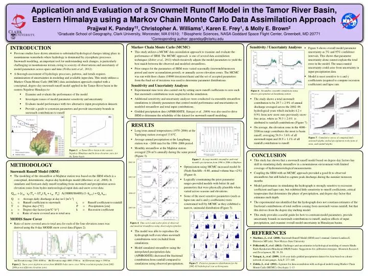
1. Prajjwal K. Panday1†, Christopher A. Williams1, Karen E. Frey1, & Molly E. Brown21Graduate School of Geography, Clark University, Worcester, MA 01610; 2 Biospheric Sciences, NASA Goddard Space Flight Center, Greenbelt, MD 20771 †Corresponding author: ppanday@clarku.edu INTRODUCTION Markov Chain Monte Carlo (MCMC) Sensitivity / Uncertainty Analyses • Figure 6 shows overall model parameter uncertainty as 5% and 95% confidence intervals. This shows that parameter uncertainty alone cannot explain the total error in the model. The unaccounted uncertainty could arise from uncertainty in input precipitation data. • Model is most sensitive to x and y coefficients (required to compute recession coefficient) and lapse rate. • This study utilizes a MCMC data assimilation approach to examine and evaluate the performance of SRM. The MCMC approach is one of several data assimilation techniques (Zobitz et al., 2011) which iteratively adjusts the model parameters to yield the best match between the observed and modeled streamflows. • Prior ranges for the parameters of SRM were varied seasonally (snowmelt/monsoon period and snow accumulation period), or annually across elevation zones. The MCMC was run with three chains (10000 iterations/chain) and the set of accepted parameters from the final set of iterations was used to determine parameter distributions. • Previous studies have drawn attention to substantial hydrological changes taking place in mountainous watersheds where hydrology is dominated by cryospheric processes. Snowmelt modeling, an important tool for understanding such changes, is particularly challenging in mountainous terrain owing to scarcity of observations and uncertainty of model parameters across space and time (Pellicciotti et al., 2012). • A thorough assessment of hydrologic processes, patterns, and trends requires minimization of uncertainties in modeling and available input data. This study utilizes a Markov Chain Monte Carlo (MCMC) data assimilation approach coupled with a conceptual, degree-day snowmelt runoff model applied in the Tamor River basin in the eastern Nepalese Himalaya to: • Examine and evaluate the performance of the model • Investigate issues of model parameter sensitivity and uncertainty • Evaluate model performance with two alternative input precipitation datasets • Provide a guide to constrain parameters and provide uncertainty bounds in snowmelt contributions to runoff Sensitivity and Uncertainty Analyses Application and Evaluation of a Snowmelt Runoff Model in the Tamor River Basin, Eastern Himalaya using a Markov Chain Monte Carlo Data Assimilation Approach • Experimental runs were also carried out by setting snow runoff coefficients to zero such that snowmelt contributions were neglected in the simulation. • Additional sensitivity and uncertainty analyses were conducted via ensemble streamflow simulations to identify parameters that control model performance and uncertainties in modeled streamflow and total input contributions. • Gridded precipitation data (APHRODITE; Yatagai et al., 2009) was also used to drive SRM to determine the reliability of the dataset for snowmelt runoff modeling. Figure 6. Streamflow ensemble simulations using observe precipitation at Lungthung station. • The study shows a total snowmelt contribution to be 29.7 ± 2.9% of annual discharge averaged across the 2002–06 hydrological years which includes 4.2 ± 0.9% from new snow onto previously snow-free areas, where as 70.3 ± 2.6% is attributed to rainfall contributions (Figure 7). • On average, the elevation zone in the 4000–5500 m range contributes the most to basin runoff, averaging 56.9 ± 3.6% of all snowmelt input and 28.9 ± 1.1% of all rainfall contribution to runoff. (a) (b) RESULTS • Long term annual temperatures (1970–2006) at the Taplejung station averaged 13.6°C. • Average annual precipitation at the Lungthung station was ~2484 mm for the 1996–2006 period. • Monthly streamflow at the Majhitar station averaged 256 m3/s annually during the same period (Figure 3). Figure 7. Cumulative curves of computed daily snowmelt depths, melted precipitation in the form of snow, and rainfall depths. Figure 1. a) Tamor River basin in the eastern Nepalese Himalaya and b) Area-elevation curve for the Tamor basin CONCLUSION Figure 3. Average monthly streamflow and total monthly precipitation from 1996 to 2006 at Majhitar • This study has shown that a snowmelt runoff model based on degree-day factors has skill in simulating daily streamflow in a mountainous environment with limited coverage of hydrometeorological measurements. • Coupling the SRM with an MCMC approach provided a good fit to observed streamflows but still failed to capture peak discharge during the summer monsoon months. • Model performance in simulating the hydrograph is strongly sensitive to recession coefficient and lapse rate, but exhibited little sensitivity to runoff coefficients, critical temperature that determines the phase of precipitation, and degree-day factor that estimates melt depth. • The experimental run identified that the hydrograph does not constrain estimates of the fractional contributions of total outflow coming from snowmelt versus rainfall, but that this derives from the degree day melting model. • This study provides a useful guide for how to constrain model parameters, provide uncertainty bounds in snowmelt contributions to runoff, analyze effects of input precipitation, and examine overall model uncertainty in Himalayan basins. 2002–03 METHODOLOGY • Optimization using MCMC increased model fit (Nash-Sutcliffe ~0.80, annual volume bias <2%) (Figure 4). • Logically constraining the prior parameter ranges provided models with better fit and parameters that were physically plausible when varied across seasons and elevations. • Some of the most sensitive parameters (such as lapse rate and x and y coefficients) were constrained well by MCMC as they exhibited a narrow, unimodaldistribution (Figure 5). Snowmelt Runoff Model (SRM) • The modeling of the streamflow at Majhitar station was based on the SRM which is a conceptual, deterministic, degree-day hydrologic model (Martinec et al., 2008). It simulates and forecasts daily runoff resulting from snowmelt and precipitation across elevation zones from hydro-meteorological input data and snow cover data. 2003–04 Qn+1 = [csn . an (Tn + ΔTn) Sn + crn . Pn] A(10000/86400) (1−kn+1) + Qn kn+1 2004–05 Q = Average daily discharge at day n+1 [m3s-1] cs = Runoff coefficient to snowmelt cr = Runoff coefficient to rainfall T = Degree days [°C] P = Precipitation [cm] a = Degree-day factor [cm°C-1d-1] k = Recession coefficient S = Ratio of snow covered area to total area 2005–06 MODIS Snow Cover Figure 4. Time series and scatter plots of observed and modeled streamflows using observed precipitation • Ratio of snow covered area to total area for each of the four elevation zones was derived using the 8-day MODIS snow cover data (Figure 2). REFERENCES • The model was able to reproduce the hydrograph well even when snowmelt contributions were excluded from simulations. • Model simulated streamflow using the interpolated precipitation data (APHRODITE) decreased the fractional contribution from rainfall compared to simulations using observed precipitation. • Martinec, J., et al. (2008). Snowmelt Runoff Model (SRM) user’s manual. Gomez-Landsea E, Bleiweiss MP (eds). New Mexico State University. • Pellicciotti, F., et al. (2012). Challenges and uncertainties in hydrological modeling of remote Hindu Kush-Karakoram-Himalayan (HKH) basins: Suggestions for calibration strategies: Mountain Research and Development, 32: 39–50. • Yatagai, A., et al. (2009). A 44-year daily gridded precipitation dataset for Asia based on a dense network of rain gauges. Sola,5: 137–140. • Zobitz, J., et al.(2011). A primer for data assimilation with ecological models using Markov Chain Monte Carlo (MCMC). Oecologia: 1–13. (a) Elevation range 2500–4000 m (b) Elevation range 4000–5500 m (c) Elevation range > 5500 m Figure 5. Posterior parameter distributions for the 2002–03 hydrological year as histograms. Figure 2. Snow cover depletion curves from MODIS 8-day snow cover 500-m resolution product from 2002–2006 across different elevation zones