Download
1 / 11
110 likes | 290 Views
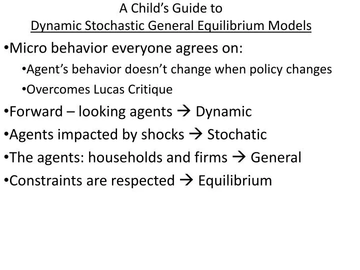
A Child’s Guide to Dynamic Stochastic General Equilibrium Models. Micro behavior everyone agrees on: Agent’s behavior doesn’t change when policy changes Overcomes Lucas Critique Forward – looking agents Dynamic Agents impacted by shocks Stochatic

E N D
A Child’s Guide to Dynamic Stochastic General Equilibrium Models Micro behavior everyone agrees on: Agent’s behavior doesn’t change when policy changes Overcomes Lucas Critique Forward – looking agents Dynamic Agents impacted by shocks Stochatic The agents: households and firms General Constraints are respected Equilibrium
The Global Great Depression: A Real Business Cycle?Review of Economic Dynamics, January 2000
P AS • Observed fluctuations must be owing to AS shocks • Factor inputs and productivity • “Intertemporal” labor-leisure substitution AD The German Slump as a Real Business Cycle Y Rational expectations Real business cycles (RBC) Dynamic (Stochastic) General Equilibrium Growth Model DSGE applied to short-run fluctuations to explain Great Depression by Fisher and Hornstein Representative agents weigh future utility when deciding how much to work and how much to save/invest at present They ignore monetary impacts … “Money lagged output” Recall Voth: lower interest rate might have stimulated investment, output and employment A Major critique of RBC-theory – the Great Depression Lucas/Prescott: Gone fish’n’ ??? German slump: Hoffmann data Ritschl data 8 – hour day: a productivity shock
Fisher – Hornstein: DGE model of Germany, 1928-37 • All per capita variables relative to real gdp trend (in equilibrium, they should grow at same rate) • Measure total factor productivity (TFP) as Solow residual: Y = A Kα L(1- α) dA/A = TFP growth = dY/Y – αdK/K – (1 - α) dL/L • Ignore M1 … it lagged Y • Output determined by Cobb-Douglas production function Y = A k.25 [γtn].75 • Labor share of income averaged ¾ • Technology advanced at 1.87% annual rate (γ) • Profit maximizing firm hires factors (n and x) so MPL = w and MPK = r Note • Wages set by collective bargaining and arbitration Political Wage Wages too High? (Borchardt) • Bruening austerity policy...he raised taxes and cut spending • Nazis broke unions (1933) – set maximum wages and limited mobility Bruening lowered civil servant wages and tried to reduce private sector wages • Nazi expansion with limits to consumption Military Keynesianism?
Fisher – Hornstein Simulations • Response of employment, output, consumption, investment and real wage to alternative values of productivity (trend or actual), fiscal policy (trend or actual), and real wage (market clearing or actual) I – Actual productivity with trend fiscal stance and market clearing wage Real wage should have declined to clear labor market, not risen, in early years of German depression II – Actual fiscal policy with trend TFP and market clearing real wage Predict not nearly as much contraction of employment, output, consumption and investment as actually occurred from 1928 – 1932. III – Actual real wage with trend TFP and actual fiscal policy Predict less reduction in consumption than actually occurred … but otherwise generate patterns close to actual Combinations of actual real wages, Bruening fiscal austerity followed by Nazi expansion, and actual TFP trace decline in investment, output and employment but fail to predict sharp decline in consumption in downturn and failure to recover in upturn. • More research is called for.
German Interwar Economic Pathologies: An Overview Lost War and Revolution Distributional Conflict +8 – Hour Day Desperate Government Hyperinflation Stabilization Monetary Constraints Outsized Wages Reduced Investment Depression and Slump Nazi Revolution/Constraints Broken Wages Down Government Spending Up (military Keynesianism) “Recovery”