Download
1 / 17
200 likes | 434 Views
Dynamic Models. Lecture 13. Dynamic Models: Introduction. Dynamic models can describe how variables change over time or explain variation by appealing to mechanisms. The informatics systems described in this lecture focus on explanatory models derived from scientific knowledge.

E N D
Dynamic Models Lecture 13
Dynamic Models: Introduction Dynamic models can describe how variables change over time or explain variation by appealing to mechanisms. The informatics systems described in this lecture focus on explanatory models derived from scientific knowledge. There are several approaches to dynamic modeling, but we focus on systems that represent models based on • qualitative process theory, • differential and algebraic equations, and • agent-level behavior. Although not exhaustive, these approaches cover a broad range of modeling techniques
Dynamic Models: Historical Use • Limits to Growth • Others…
Garp3 The Garp3 environment supports qualitative process models, which emphasize processes and entities. The entities in this hierarchy have properties altered during simulation. A model is a collection of model fragments that define its dynamics. Scenarios give the starting values for the properties of entities. This scenario starts with a small number of green frogs. The model explains frog population dynamics.
Garp3: Model Fragments This process defines the positive population growth model fragment. The growth rate of a population directly influences its size. Additionally, population size is proportional to the growth rate. Here the growth rate is fixed to Plus, which is any positive number. This entity definition states that a population must have the property Number of.
Garp3: Simulation Given a starting scenario, Garp3 models produce envisionments of the state space. Each state differs in its values for entity properties. These trajectories show the properties in states 3, 4, and 6. Population growth was forced to be positive. The number of frogs increases over time as one would expect.
STELLA The STELLA environment supports system dynamics models based on Forrester diagrams. A stock accumulates quantities (e.g., fish, chemicals, people) A flow controls the movement of quantities between stocks. A converter carries out algebraic transformations of quantities. Quantities may flow from infinite sources or to infinite sinks.
STELLA: Model Construction Model construction in STELLA involves laying out the visual components and specifying their properties. The being born flow is defined as: Population * birth fraction The parameter birth fraction is set to 0.5, but may be tuned.
STELLA: Model Simulation Some of the equations from the Easter Island model. Simulated trajectories from the Easter Island model.
NetLogo The NetLogo environment supports agent-based models, which stress individual and environmental interaction. NetLogo models are represented in a procedural language, but are controlled by custom graphical interfaces. Controls are on the left. Variable trajectories are displayed on the bottom. The environment and agents appear on the right. This model explores the social dynamics of rebellion.
NetLogo: Model Construction This example shows the code that controls the interaction between a cop and an agent in the same region. The cop will arrest a nearby rebellious (active) agent, who will go to jail for a random amount of time. ;; COP BEHAVIOR to enforce if any? (agents-on neighborhood) with [active?] [ ;; arrest suspect let suspect one-of (agents-on neighborhood) with [active?] ask suspect [ set active? false set jail-term random max-jail-term ] move-to suspect ;; move to patch of the jailed agent ] end
NetLogo: Simulation The agent window shows: • jailed agents as dark circles, • active agents as red circles, • quiet agents as green circles, and • cops as blue triangles. NetLogo also displays trajectories for the various agent populations.
Prometheus The Prometheus environment supports quantitative process models which emphasize variables and processes. The light availability process calculates light’s limiting factor on plant growth. Death, grazing, and growth processes control the dynamics of the phytoplankton population. Phytoplankton affects grazing rate and nitrate uptake.
Prometheus: Model Representation The graphical representation shows causal interactions. Corresponding differential and algebraic equations.
Prometheus: Editing and Simulating Models Scientists can instantiate processes from a library. Simulating models produces a trajectory for each variable.
Dynamic Models: Summary The informatics systems discussed in this lecture covered several modeling styles: • Garp3 is unique in that it represents dynamics as discrete state transitions; • STELLA treats the world as quantities of stuff that undergo constant transformation; • Prometheus represents the world in terms of mechanisms that drive system evolution; and • NetLogo distinctively focuses on individual interactions as opposed to aggregate entities or quantities. These different modeling paradigms reflect and influence scientific thinking about dynamical systems.