Download
1 / 1
10 likes | 294 Views
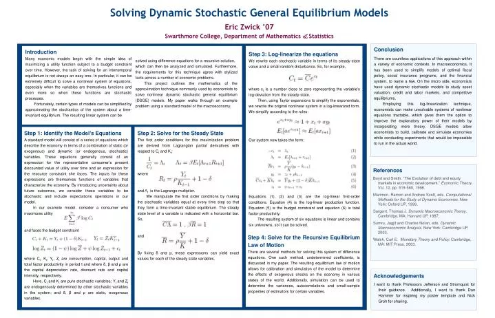
Solving Dynamic Stochastic General Equilibrium Models Eric Zwick ’07 Swarthmore College, Department of Mathematics & Statistics. Conclusion

E N D
Solving Dynamic Stochastic General Equilibrium Models Eric Zwick ’07 Swarthmore College, Department of Mathematics & Statistics Conclusion There are countless applications of this approach within a variety of economic contexts. In macroeconomics, It has been used to simplify models of optimal fiscal policy, social insurance programs, and the financial system, to name a few. On the micro side, economists have used dynamic stochastic models to study asset valuation, credit and labor markets, and competitive equilibriums. Employing this log-linearization technique, economists can make unsolvable systems of nonlinear equations tractable, which gives them the option to improve the explanatory power of their models by incorporating more theory. DSGE models allow economists to build, calibrate and simulate economies while conducting experiments that would be impossible to run in the actual world. Introduction Many economic models begin with the simple idea of maximizing a utility function subject to a budget constraint over time. However, the task of solving for an intertemporal equilibrium is not always an easy one. In particular, it can be extremely difficult to solve a nonlinear system of equations, especially when the variables are themselves functions and even more so when these functions are stochastic processes. Fortunately, certain types of models can be simplified by approximating the stochastics of the system about a time- invariant equilibrium. The resulting linear system can be Step 3: Log-linearize the equations We rewrite each stochastic variable in terms of its steady-state value and a small random disturbance. So, for example, where ct is a number close to zero representing the variable’s log-deviation from the steady-state. Then, using Taylor expansions to simplify the exponentials, we rewrite the original nonlinear system in a log-linearized form. We simplify according to the rules: Our system now takes the form: Equations (1), (2) and (3) are the log-linear first-order conditions. Equation (4) is the log-linear production function. Equation (5) is the budget constraint and equation (6) is total factor productivity. The resulting system of six equations is linear and contains six unknowns, so it can be solved. solved using difference equations for a recursive solution, which can then be analyzed and simulated. Furthermore, the requirements for this technique agree with stylized facts across a number of economic problems. This project outlines the mathematics of the approximation technique commonly used by economists to solve nonlinear dynamic stochastic general equilibrium (DSGE) models. My paper walks through an example problem using a standard model of the macroeconomy. Step 1: Identify the Model’s Equations A standard model will consist of a series of equations which describe the economy in terms of a combination of static (or exogenous) and dynamic (or endogenous, stochastic) variables. These equations generally consist of an expression for the representative consumer’s present discounted value of utility over time and an expression for the resource constraint she faces. The inputs for these expressions are themselves functions of variables that characterize the economy. By introducing uncertainty about future outcomes, we consider these variables to be stochastic and include expectations operations in our model. In our example model, consider a consumer who maximizes utility and faces the budget constraint where Ct, Kt, Yt, Zt are consumption, capital, output and total factor productivity in period t and where δ, β and ρ are the capital depreciation rate, discount rate and capital intensity, respectively. Here, Ct and Kt are pure stochastic variables; Yt and Zt are endogenously determined by other stochastic variables in the system; and δ, β and ρ are static, exogenous variables. Step 2: Solve for the Steady State The first order conditions for this maximization problem are derived from Lagrangian partial derivatives with respect to Ct and Kt: where and Λt is the Lagrange multiplier. We manipulate the first order conditions by making the stochastic variables equal at every time step so that they form a time-invariant stable equilibrium. The steady state level of a variable is indicated with a horizontal bar. So, and By fixing δ and β, these expressions can yield exact values for each of the steady state variables. References Boyd and Smith. “The Evolution of debt and equity markets in economic development.” Economic Theory. Vol. 12, pp. 519-560, 1998. Marimon, Ramon and Andrew Scott, eds. Computational Methods for the Study of Dynamic Economies. New York: Oxford UP, 1999. Sargent, Thomas J. Dynamic Macroeconomic Theroy. Cambridge, MA: Harvard UP, 1987. Sumru, Jagjit and Charles Nolan, eds. Dynamic Macroeconomic Analysis. New York: Cambridge UP, 2003. Walsh, Carl E. Monetary Theory and Policy. Cambridge, MA: MIT Press, 2003. Step 4: Solve for the Recursive Equilibrium Law of Motion There are several methods for solving this system of difference equations. One such method, undetermined coefficients, is discussed in my paper. The resulting equilibrium law of motion allows for calibration and simulation of the model to determine the effects of exogenous shocks on the economy in various states of the world. Additionally, simulation can be used to determine the variances, autocorrelations and small-sample properties of estimators for certain variables. Acknowledgements I want to thank Professors Jefferson and Stromquist for their guidance. Additionally, I want to thank Dan Hammer for inspiring my poster template and Nick Groh for sharing.