Download
1 / 53
540 likes | 758 Views
William Greene Stern School of Business New York University. Stochastic Frontier Models. 0 Introduction 1 Efficiency Measurement 2 Frontier Functions 3 Stochastic Frontiers 4 Production and Cost 5 Heterogeneity 6 Model Extensions 7 Panel Data 8 Applications. Where to Next?.

E N D
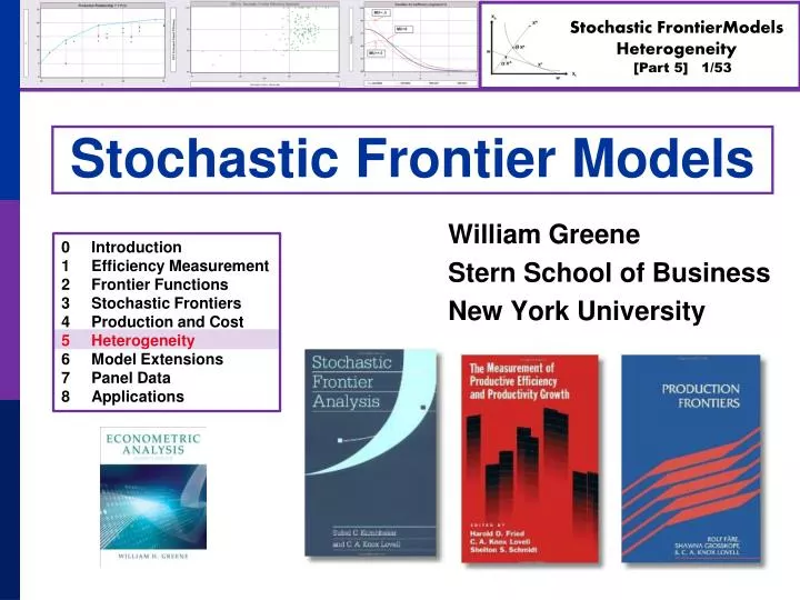
William Greene Stern School of Business New York University Stochastic Frontier Models 0 Introduction 1 Efficiency Measurement 2 Frontier Functions 3 Stochastic Frontiers 4 Production and Cost 5 Heterogeneity 6 Model Extensions 7 Panel Data 8 Applications
Where to Next? • Heterogeneity: “Where do we put the z’s?” • Other variables that affect production and inefficiency • Enter production frontier, inefficiency distribution, elsewhere? • Heteroscedasticity • Another form of heterogeneity • Production “risk” • Bayesian and simulation estimators • The stochastic frontier model with gamma inefficiency • Bayesian treatments of the stochastic frontier model • Panel Data • Heterogeneity vs. Inefficiency – can we distinguish • Model forms: Is inefficiency persistent through time? • Applications
Observable Heterogeneity • As opposed to unobservable heterogeneity • Observe: Y or C (outcome) and X or w (inputs or input prices) • Firm characteristics or environmental variables. Not production or cost, characterize the production process. • Enter the production or cost function? • Enter the inefficiency distribution? How?
Shifting the Outcome Function Firm specific heterogeneity can also be incorporated into the inefficiency model as follows: This modifies the mean of the truncated normal distribution yi = xi + vi - ui vi ~ N[0,v2] ui = |Ui| where Ui ~ N[i, u2], i = 0 + 1zi,
One Step or Two Step 2 Step: 1. Fit Half or truncated normal model, 2. Compute JLMS ui, regress ui on zi Airline EXAMPLE: Fit model without POINTS, LOADFACTOR, STAGE 1 Step: Include zi in the model, compute ui including zi Airline example: Include 3 variables Methodological issue: Left out variables in two step approach.
One vs. Two Step 0.8 0.9 1.0 Efficiency computed without load factor, stage length and points served. Efficiency computed with load factor, stage length and points served.
Unobservable Heterogeneity • Parameters vary across firms • Random variation (heterogeneity, not Bayesian) • Variation partially explained by observable indicators • Continuous variation – random parameter models: Considered with panel data models • Latent class – discrete parameter variation
Latent Class Efficiency Studies • Battese and Coelli – growing in weather “regimes” for Indonesian rice farmers • Kumbhakar and Orea – cost structures for U.S. Banks • Greene (Health Economics, 2005) – revisits WHO Year 2000 World Health Report • Kumbhakar, Parmeter, Tsionas (JE, 2013) – U.S. Banks.
Latent Class Application Estimates of Latent Class Model: Banking Data
Inefficiency? • Not all agree with the presence (or identifiability) of “inefficiency” in market outcomes data. • Variation around the common production structure may all be nonsystematic and not controlled by management • Implication, no inefficiency: u = 0.
Nursing Home Costs • 44 Swiss nursing homes, 13 years • Cost, Pk, Pl, output, two environmental variables • Estimate cost function • Estimate inefficiency
A Two Class Model • Class 1: With Inefficiency • logC = f(output, input prices, environment) + vv + uu • Class 2: Without Inefficiency • logC = f(output, input prices, environment) + vv • u = 0 • Implement with a single zero restriction in a constrained (same cost function) two class model • Parameterization: λ = u /v = 0 in class 2.
LogL= 464 with a common frontier model, 527 with two classes
Heteroscedasticity in v and/or u yi = ’xi + vi - ui Var[vi| hi] = v2gv(hi,) = vi2 gv(hi,0) = 1, gv(hi,) = [exp(’hi)]2 Var[Ui | hi] = u2gu(hi,)= ui2 gu(hi,0) = 1, gu(hi,) = [exp(’hi)]2
Unobserved Endogenous Heterogeneity • Cost = C(p,y,Q), Q = quality • Quality is unobserved • Quality is endogenous – correlated with unobservables that influence cost • Econometric Response: There exists a proxy that is also endogenous • Omit the variable? • Include the proxy? • Question: Bias in estimated inefficiency (not interested in coefficients)
Simulation Experiment • Mutter, et al. (AHRQ), 2011 • Analysis of California nursing home data • Estimate model with a simulated data set • Compare biases in sample average inefficiency compared to the exogenous case • Endogeneity is quantified in terms of correlation of Q(i) with u(i)
A Simulation Experiment Conclusion: Omitted variable problem does not make the bias worse.
Sample Selection Modeling Switching Models: y*|technology = bt’x + v –u Firm chooses technology = 0 or 1 based on c’z+e e is correlated with v Sample Selection Model: Choice of organic or inorganic Adoption of some technological innovation
Early Applications • Heshmati A. (1997), “Estimating Panel Models with Selectivity Bias: An Application to Swedish Agriculture”, International Review of Economics and Business 44(4), 893-924. • Heshmati, Kumbhakar and Hjalmarsson Estimating Technical Efficiency, Productivity Growth and Selectivity Bias Using Rotating Panel Data: An Application to Swedish Agriculture • Sanzidur Rahman Manchester WP, 2002: Resource use efficiency with self-selectivity: an application of a switching regression framework to stochastic frontier models:
Sample Selection in Stochastic Frontier Estimation • Bradford et al. (ReStat, 2000):“... the patients in this sample were not randomly assigned to each treatment group. Statistically, this implies that the data are subject to sample selection bias. Therefore, we utilize astandard Heckman two-stage sample-selection process, creating an inverse Mill’s ratio from a first-stage probit estimator of the likelihood of CABG or PTCA. This correction variable is included in the frontier estimate....” • Sipiläinen and Oude Lansink (2005) “Possible selection bias between organic and conventional productioncan be taken into account [by] applying Heckman’s (1979) two step procedure.”
Two Step Selection • Heckman’s method is for linear equations • Does not carry over to any nonlinear model • The formal estimation procedure based on maximum likelihood estimation • Terza (1998) – general results for exponential models with extensions to other nonlinear models • Greene (2006) – general template for nonlinear models • Greene (2010) – specific result for stochastic frontiers
A Sample Selected SF Model di = 1[′zi + wi > 0], wi ~ N[0,12] yi = ′xi + i, i ~ N[0,2] (yi,xi) observed only when di = 1. i = vi- ui ui = |uUi| = u |Ui| where Ui ~ N[0,12] vi = vVi where Vi ~ N[0,12]. (wi,vi) ~ N2[(0,1), (1, v, v2)]
Alternative Approach Kumbhakar, Sipilainen, Tsionas (JPA, 2008)
Simulated Log Likelihood for a Stochastic Frontier Model The simulation is over the inefficiency term.
WHO Efficiency Estimates OECD Everyone Else