Download

1 / 42
420 likes | 540 Views
Theories and Methods of the Business Cycle. Part 1: Dynamic Stochastic General Equilibrium Models IV. A New Neoclassical Synthesis? Jean-Olivier HAIRAULT , Professeur à Paris I Panthéon-Sorbonne et à l’Ecole d’Economie de Paris (EEP). 1. Introduction.

E N D
Theories and Methods of the Business Cycle. Part 1: Dynamic Stochastic General Equilibrium Models IV. A New Neoclassical Synthesis? Jean-Olivier HAIRAULT, Professeur à Paris I Panthéon-Sorbonne et à l’Ecole d’Economie de Paris (EEP)
1. Introduction • The RBC theory is at odds with the neoclassical synthesis • Real shocks vs. Monetary shocks • Optimal vs. Suboptimal fluctuations • RBC theory has not totally convinced that technology shocks can alone drive the business cycle. The internal mechanisms of the neoclassical growth model does not lead to fluctuations totally consistent with the stylized facts when calibration is seriously done. • The correlation between hours and labor productivity is too high • The response of output does not display a hump-shaped profile • How to reconcile theory with the numerous empirical works which show the non-neutrality of money (in particular in the VAR framework)? Gali [1989], Quarterly Journal of Economics
1. Introduction • Along the development of RBC theory in the 80’s, keynesianism was looking for micro-foundations • How to get market failures when agents are assumed to optimize? • Imperfect information, imperfect competition, strategic behaviors,…New-Keynesianism based on real and nominal rigidities. Ball and Romer [1990], Review of Economic Studies • Non-walrasian features in the good market (monopolistic competition), the labor market (search frictions), the credit market (adverse selection and moral hazard) • Mainly theoretical works as new-keynesianism has to address the Lucas’ critique. • What a challenge to overcome RBC theory with their own methodology! • The 90’s was the decade during which a new neoclassical synthesis occurs: intertemporal choices and strategic behaviors
2. Equilibrium unemployment • Employment volatility represents 70% of total hours volatility • Hours indivisibility à la Hansen [1985] • Do efficiency wages better explain the relative volatility of hours to labor productivity? Danthine and Donaldson [1990], European Economic Review. Employment is not volatile enough in their model • Efficiency wages are rigid in the sense they do not clear the labor market, but they are elastic to technology shocks. • Fluctuations generated by the model are essentially the same as those of the RBC canonical model.
2. Equilibrium unemployment • Equilibrium unemployment, Pissarides [1990], Equilibrium unemployment theory, Basil Blackwell • Hirings take time as there is imperfect information in the process of search: search unemployment • Search frictions could explain the persistence of fluctuations • Merz [1995], Journal of Monetary Economics, Andolfatto [1996], American Economic Review
2. Equilibrium unemployment • Hirings depend on vacancies (V) and unemployed people (U), but also the search intensity (e) of these latter. • The participation rate is constant and exogenous. • The probability to have a job is: • The probability to contact a worker: • There are externalities in the search process • p depends positively on the number of vacancies (complementarity) and negatively on the number of unemployed workers (congestion) • q depends negatively on the number of vacancies and positively on the number of unemployed workers (congestion)
2. Equilibrium unemployment • The dynamics of employment depends on hirings (a combination of unemploment and vacancy) and on firings (a fixed proportion s of the employment stock)
2. Equilibrium unemployment • Representative household (risk-sharing due to the large scale of the household) • First order conditions are the same as those in the canonical RBC model, except there is no labor supply, no partipation decision and hours are negociated between households and firms (as wage)
2. Equilibrium unemployment • The production function is traditional and combines total hours and capital. • Firm labor demand is no more static, as they invest in vacancies. The firm program is now intertemporal. • Labor demand is now determined by the intertemporal condition:
2. Equilibrium unemployment • Bargaining over hours and wage • Nash criterion • With • is the bargaining power of firms. In Andolfatto [1996], it is equal to the elasticity relative to vacancy in the matching function. In this case, the bargaining leads to the first best allocation as demonstrated by Hosios [1990], Review of Economic Studies. • Given the existence of search frictions, fluctuations are not necessarily sub-optimal. This is why Andolfatto [1996] solves the planner program.
2. Equilibrium unemployment • Stylized facts : standart deviation in the first line, correlation with output in the second line • Andolfatto [1996] • The wage is no longer equal to labor productivity and the labor share is variable and counter-cyclical. The variance of output is obtained without infinite labor elasticity, but results from its higher persistence. • But the correlation between hours and wage is not replicated. • Increasing the volatility of employment by giving more bargaining power to firms as their response to technology shocks will then be more elastic.
2. Equilibrium unemployment • Productivity cycle and Beveridge curve • Stylized facts • Model’s predictions: the productivity cycle is not replicated contrary to the Beveridge curve
3. Perfect Insurance • Complete markets: perfect risk sharing • B is the amount of insurance whose price is tau. • 1-alpha= s for employed workers; 1-alpha = 1-p for unemployed workers • Two insurance schemes: profit = • The budgetary constraints:
3. Perfect Insurance • First-order conditions: • Risk-sharing condition • For s = n, u • These conditions imply that the capital choices are identical whatever their employment status. For separable utility fonction, consumptions are the same, and the unemployed workers are better off. See Chéron and Langot [2002], Review of Economic Dynamics for a case where their welfare is lower than that of employed workers.
3. Perfect Insurance • Given these optimal choices, the budgetary constraints can be rewritten as follows: • It can be noticed that: • The representative household program is then:
4. Monopolistic competition and nominal rigidities • Considering VAR studies (following the seminal article of Sims [1980], Econometrica), money supply shocks would impact the output. J. Gali [1992], Quarterly Journal of Economics, Bec and Hairault [1993], Annales d’Economie et Statistiques [1993] • Taking into account money supply shock in DSGE models implies to have money demand theoretical foundations: Why do we hold money ? Old issue in economics… • Money reduces transaction or search costs in the good market: Kiyotaki and Wright [1989], Journal of Political Economy • More tractable in DSGE models, cash-in-advance constraint can be added in the household program, Cooley and Hansen [1989], American Economic Review: • Without any nominal rigidities, this approach fails to generate a positive and strong response of output after a positive monetary (supply) shock. Only the inflation tax propagation mechanism which is a negative wealth effect: positive response of labour supply and output, but very weak effects.
4. Monopolistic competition and nominal rigidities • (Inflation tax +) nominal rigidities: prices are rigid due to menu costs (New-Keynesian approach) (an alternative: rigidity of the nominal wage due to the existence of wage contracts) • This implies to consider imperfect competition in the good market: monopolistic competition in the line of Blanchard and Kiyotacki [1897], American Economic Review • Nominal rigidities + monopolistic competition in DSGE: Hairault and Portier [1993], European Economic Review
4. Monopolistic competition and nominal rigidities • Firms have monopoly power due to good differentiation. • Prices include a mark-up over the marginal cost. • Firms maximize profit by taking into account the effect of prices on the good demand. • The demand for good j is a proportion of the total demand which depends on the relative price of good j: • The total demand for good j is then:
4. Monopolistic competition and nominal rigidities • The nominal profit of firm j is: • Due to the presence of adjustment costs on prices, firm choices are now intertemporal:
4. Monopolistic competition and nominal rigidities • The first-order conditions are : • Prices are not equalized to marginal costs:
4. Monopolistic competition and nominal rigidities • Money is introduced into the utility function:
4. Monopolistic competition and nominal rigidities • The first-order conditions are: • The money supply process is:
4. Monopolistic competition and nominal rigidities • The Solow Residual is no longer a pure measure of technology. The factor elasticities are not consistently measured by factor shares in total revenues due to the existence of markups. • The naive SR is contamined by money supply shocks as these latter make markups counter-cyclical in the business cycle • After a money supply shock, firms want to increase prices in order to leave unchanged their mark-up. As there exist adjustment costs on prices, prices do not increase as much as invariant mark-up would imply. Markups are weaker than at the steady state.
4. Monopolistic competition and nominal rigidities • Stylized facts • Model’s predictions
5. Financial imperfections • Limited participation and money supply shocks • Fuerst [1992], Journal of Monetary Economics, Christiano and Eichenbaum [1992], American Economic Review • The nominal and real interest rates decline after a positive monetary shock in empirical studies
5. Financial imperfections • The nominal and real interest rates decline after a positive monetary shock since the supply of deposits is pre-determined • Firms rent wages R Dd, Ds
5. Financial imperfections • Financial Accelerator, Carlstrom and Fuerst [1997], American Economic Review, Bernanke, Gertler and Gilchrist, Handbook of Macroeconomics • Entrepreneurs have access to a risky project. Lenders have no information about the ex-post return. They have to pay a verification cost. • The optimal contract is then a debt contract. The debtor interest rate depends on the entrepreneur’s wealth. • Serial correlation of output growth depends on the agency costs:
6. Sunspot and fluctuations • Self-fulfilling propheties, Farmer and Guo [1994], Journal of Economic Theory • Animal spirits at the heart of the business cycle • Extrinsic shocks vs. Shocks on fundamentals • Indeterminacy of the equilibrium: too many eigenvalues inferior to 1 (more than the number of pre-determined variables). • Sunspot equilibria can arise in this case. • This approach must be distinguished from news about the future of some fundamentals, see Hairault, Langot and Portier [1997], Journal of Economic, Dynamics and Control, Beaudry and Portier [2006], American Economic Review
6. Sunspot and fluctuations • Final good is produced by using intermediated inputs • Production of these inputs under increasing return to scale and monopolistic competition • The reduced form of the model is : • with
6. Sunspot and fluctuations • If the labor elasticity is small enough relative to a, ie the labor demande curve is increasing with a slop superior to that of the labor supply curve, the eigenvalues are strictly inferior to one and sunspot equilibria exist
7. Business cycle costs • Stabilization of business cycle? What does it mean in the DSGE framework? • Welfare criterion must be considered, and not volatility criterion, especially the output volatility • Business cycle costs are very small in terms of stationary consumption; eliminating all fluctuations is equivalent in welfare units to 0.008% of the steady state consumption, Lucas [1987], Models of Business Cycles, Basil Blackwell. • This implies that the distorsions introduced by the stabilization policy must be very small too. • Harberger triangles could be much more important than Okun gaps, Greenwood and Huffman [1991], Journal of Monetary Economics. • « I argue in the end that, based on what we know now, it is unrealistic to hope for gains larger than a tenth of a percent from better countercyclical policy » Lucas [2003], American Economic Review
7. Business cycle costs • Reis [2007]