Download
1 / 23
230 likes | 234 Views
Predicting species distributions for New England invasives. Explanatory data layers: Field collected information: habitat/community type, canopy closure, slope aspect, soil moisture regime

E N D
Explanatory data layers: • Field collected information: habitat/community type, canopy closure, slope aspect, soil moisture regime • Climate variables: Mean annual precipitation, Mean annual snow fall, Mean annual min & max temperatures, Annual record extreme min & max temperature, Mean annual temperature, Mean length of frost free period, Mean number of growing degree days, Mean annual number of heating degree days: 2 km grid scale. • Topographic variables: DEM - average elevation for 2km grid cell, DEM – range, high and low values for 2km grid cell. • Road influences: Distance to Road (for each IPANE plot point), Length of Roads within each 2km grid cell. • Landuse – landcover: percent land cover of each of 9 classes resampled from 30m resolution to 2 km.
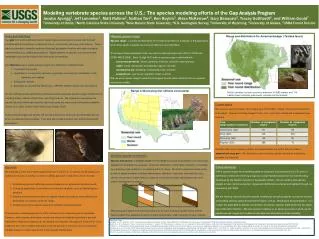
IPANE data are used for predictive modeling. Here is the predicted spread of Celastrus orbiculatus (from dark areas to light areas) in New England. The uncertainty (variance) is also measured in the predictive model (darker areas are most uncertain). Celastrus orbiculatus Oriental bittersweet Example of modeled invasive distribution at the regional scale: Oriental bittersweet
Is there an effects of land-use or land-use change on the distribution of invasive species in the New England landscape?
Quantifying land-use change in the landscape over the past 70 years from aerial photography in Connecticut 2000 1970 1951 1934
Procedure • Process historical aerial photographs – create geo-corrected mosaic images of 5 different time periods. • Digitize land use features - visual interpretation of aerial mosaics using a suite of LULC categories. • Create a stratified random sampling scheme - Generate 50+ random points for each change category. • Sampling - based upon the IPANE plot protocols
LULC Change Categories 1. Forest - No Change 2. Cultivated Fields - No change 3. Pasture/Meadow - No change 4. Residential/Commercial - No change 5. Abandoned fields to Forest 6. Cultivated fields to Forest 7. Pasture/Meadow to Forest 8. Cultivated Fields to Abandoned to Forest 9. Pasture/Meadow to Abandoned to Forest 10. Cultivated fields to Abandoned fields 11. Pasture/Meadow to Abandoned fields 12. Forest to Residential/Commercial 13. Cultivated fields to Residential/Commercial 14. Pasture to Residential/Commercial 15. Abandoned fields to Residential/Commercial 16. Abandoned fields to Forest to Residential/Commercial No Change Agricultural Fields Reverted to Forest Abandoned Fields as of 2003 Conversion to Residential/ Commercial
Final Plot Points 603 in Total: 507 Random, 96 Opportunistic
Presence of One or More Invasive Species All Plots: 363 / 603 or 60.2% Random Plots: 288 / 507 or 55.4%
C. orbiculatus: 251 out of 603 - 41.6 % Random: 186 / 507 36.7% 1000+ : 3 100 - 999: 53 20 - 99: 100
B. thunbergii: 199 out of 603 - 33.0 % Random: 140 / 507 27.6% 1000+: 2 100 - 999: 31 20 - 99: 47
Presence/AbsenceIndividual Species by LULC Groups(From Random Plots: N = 507)
Hierarchy of Invasion ( Abundance of all species combined) 1st: Abandoned Fields as of 2003 (p = .005) 2nd: Agricultural Fields Reverted to Forest (p < .0001) 3rd: Conversion to Residential / Commercial (p < .0001) 4th: Categories with No Change
Regression models Invasive species abundance = f(environmental explanatory variables) Explanatory variables: Community type (24 IPANE categories), Habitat class (4), Canopy closure, Slope aspect, Soil moisture, LULC (12 or 5), Distance to Road, Road density, Distance to nearest building, Building density, Edge Distance (and type), Elevation, Geology, Soil type and Soil drainage class.
Explaining spatial patterns in Oriental bittersweet abundance using regression models Community type: + Aspen/birch, old fields, forest/field edge, roadsides. - Oak/pine forests. LULC type: + conversion to residental/commercial, abandoned fields, fields reverting to forest. - agricultural fields, no change, especially forest. Canopy closure: - [moderate to dense canopies] Edge distance: - Minor contribution: soils, building distance, prior vegetation cover
Explaining spatial patterns in Japanese barberry abundance using regression models Canopy closure: - [for densest canopy closure] Community type: + upland red maple, northern hardwoods, birch/aspen, old fields, open fields - agricultural fields, coniferous forests, oak/pine forests. LULC: + field reverting to forests - agricultural fields, forests Edge distance: -
Mid-Spring ADAR:A Possible Remote Sensing Search Tool for Invasives?